ML4T - 第7章第6节使用Alphalens进行分析 Alphalens Analysis

原创已于 2025-10-01 12:07:52 修改 · 1k 阅读

21 ·

CC 4.0 BY-SA版权

文章标签：

#python #开发语言

于 2025-10-01 12:03:01 首次发布

ML4T 专栏收录该内容

13 篇文章

订阅专栏

一、Load Data 加载数据

二、Linear Regression 线性回归

1. Quantiles Statistics（分组统计）

2. Returns Analysis（收益分析）

3. Information Analysis（IC 分析）

4. Turnover Analysis（换手率）

5. Rank Autocorrelation（因子稳定性）

三、Ridge Regression 岭回归

四、Lasso Regression 套索回归

参考：https://github.com/stefan-jansen/machine-learning-for-trading/blob/main/07_linear_models/06_evaluating_signals_using_alphalens.ipynb

一、Load Data 加载数据

首先需要安装对应的库

! pip install alphalens-reloaded

# 原版已不再维护,推荐使用“社区重载版（alphalens-reloaded）”

import warnings
warnings.filterwarnings('ignore')

from pathlib import Path
import pandas as pd
from alphalens.tears import create_summary_tear_sheet
from alphalens.utils import get_clean_factor_and_forward_returns

idx = pd.IndexSlice

with pd.HDFStore('data.h5') as store:
    lr_predictions = store['lr/predictions']
    lasso_predictions = store['lasso/predictions']
    lasso_scores = store['lasso/scores']
    ridge_predictions = store['ridge/predictions']
    ridge_scores = store['ridge/scores']

# DATA_STORE = Path('..', 'data', 'assets.h5')
DATA_STORE = Path('data', 'assets.h5')  # change to the real path 修改到真实路径

def get_trade_prices(tickers, start, stop):
    prices = (pd.read_hdf(DATA_STORE, 'quandl/wiki/prices').swaplevel().sort_index())
    prices.index.names = ['symbol', 'date']
    prices = prices.loc[idx[tickers, str(start):str(stop)], 'adj_open']
    return (prices
            .unstack('symbol')
            .sort_index()
            .shift(-1)
            .tz_localize('UTC'))

def get_best_alpha(scores):
    return scores.groupby('alpha').ic.mean().idxmax()

def get_factor(predictions):
    return (predictions.unstack('symbol')
            .dropna(how='all')
            .stack()
            .tz_localize('UTC', level='date')
            .sort_index())

注意文件路径要选对：数据来源于前面几节

# DATA_STORE = Path('..', 'data', 'assets.h5')

DATA_STORE = Path('data', 'assets.h5') # change to the real path 修改到真实路径

get_trade_prices 函数：

功能：从 HDF5 数据存储中读取股票的历史价格数据，并返回指定时间段和调整后的开盘价。

get_best_alpha 函数：

功能：从一组分数中选择最佳的 alpha 值。

get_factor 函数：

功能：处理预测数据，将其转换为因子格式，并进行一些数据清洗和格式化。

二、Linear Regression 线性回归

lr_factor = get_factor(lr_predictions.predicted.swaplevel())
lr_factor.head()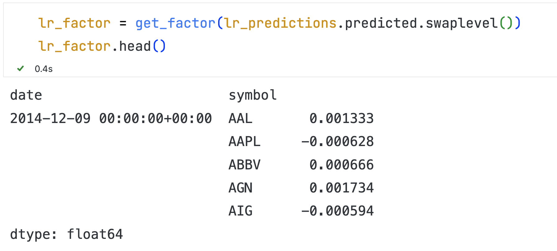

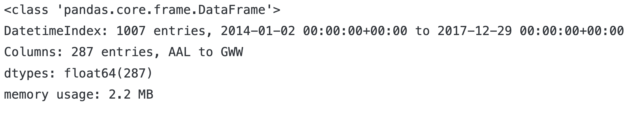
tickers = lr_factor.index.get_level_values('symbol').unique()

trade_prices = get_trade_prices(tickers, 2014, 2017)
trade_prices.info()

lr_factor_data = get_clean_factor_and_forward_returns(factor=lr_factor,
                                                      prices=trade_prices,
                                                      quantiles=5,
                                                      periods=(1, 5, 10, 21))
lr_factor_data.info()

结果：

Dropped 0.0% entries from factor data: 0.0% in forward returns computation and 0.0% in binning phase (set max_loss=0 to see potentially suppressed Exceptions).
max_loss is 35.0%, not exceeded: OK!
<class 'pandas.core.frame.DataFrame'>
MultiIndex: 73812 entries, (Timestamp('2014-12-09 00:00:00+0000', tz='UTC'), 'AAL') to (Timestamp('2017-11-29 00:00:00+0000', tz='UTC'), 'XOM')
Data columns (total 6 columns):
 #   Column           Non-Null Count  Dtype  
---  ------           --------------  -----  
 0   1D               73812 non-null  float64
 1   5D               73812 non-null  float64
 2   10D              73812 non-null  float64
 3   21D              73812 non-null  float64
 4   factor           73812 non-null  float64
 5   factor_quantile  73812 non-null  int64  
dtypes: float64(5), int64(1)
memory usage: 3.7+ MB

画图并分析

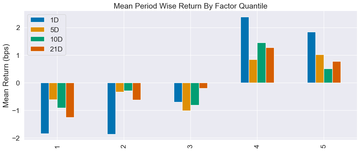
Alphalens 的 create_summary_tear_sheet 负责把单个因子拆成 5 组（quantiles）做业绩/IC/换手分析

create_summary_tear_sheet(lr_factor_data);
# 说明可以参考：alphalens入门篇  https://blog.csdn.net/u011331731/article/details/88314459
# 分析结论：短线有点信号，长线更稳，但都不强； turnover 高，费用吃利润，适合当排序信号，不适合单独对冲。

Quantiles Statistics

	min	max	mean	std	count	count %
factor_quantile
1	-0.043757	0.009896	-0.002980	0.004034	14982	20.297513
2	-0.014429	0.012193	-0.000901	0.003243	14666	19.869398
3	-0.012309	0.013843	0.000169	0.003228	14516	19.666179
4	-0.011109	0.016001	0.001188	0.003352	14666	19.869398
5	-0.009576	0.035734	0.003144	0.004032	14982	20.297513

Returns Analysis

	1D	5D	10D	21D
Ann. alpha	0.048	0.017	0.019	0.020
beta	-0.017	-0.068	-0.058	0.041
Mean Period Wise Return Top Quantile (bps)	1.842	1.016	0.514	0.778
Mean Period Wise Return Bottom Quantile (bps)	-1.847	-0.613	-0.910	-1.259
Mean Period Wise Spread (bps)	3.689	1.652	1.433	2.028

Information Analysis

	1D	5D	10D	21D
IC Mean	0.019	0.017	0.019	0.023
IC Std.	0.178	0.165	0.172	0.156
Risk-Adjusted IC	0.107	0.100	0.111	0.148
t-stat(IC)	2.940	2.745	3.053	4.045
p-value(IC)	0.003	0.006	0.002	0.000
IC Skew	-0.093	0.031	-0.158	-0.142
IC Kurtosis	-0.212	-0.053	-0.107	-0.231

Turnover Analysis

	1D	5D	10D	21D
Quantile 1 Mean Turnover	0.300	0.527	0.630	0.747
Quantile 2 Mean Turnover	0.516	0.705	0.758	0.797
Quantile 3 Mean Turnover	0.560	0.739	0.773	0.807
Quantile 4 Mean Turnover	0.515	0.704	0.756	0.789
Quantile 5 Mean Turnover	0.302	0.530	0.637	0.741

	1D	5D	10D	21D
Mean Factor Rank Autocorrelation	0.817	0.551	0.401	0.236

把单个因子拆成 5 组进行分析，通俗的例子就是：

因子值是“今天给学生按某科成绩排队”，
收益是“过几天再看他们总分涨了多少”，
拆 5 组就是“看看排在前面的学生是不是涨得最多”。

分析结论：短线有点信号，长线更稳，但都不强； turnover 高，费用吃利润，适合当排序信号，不适合单独对冲。

1. Quantiles Statistics（分组统计）

单调性良好：因子值从 Q1 到 Q5 递增，说明因子方向正确，没有反转。

2. Returns Analysis（收益分析）

alpha 低（<5%），beta 接近 0 ；市场中性，但超额收益也不高

多空对冲收益（spread） 1D 最高，但 5D/10D 下降，21D 略有回升。
收益不大，1D 的 3.7bps 扣掉交易成本（双边 ~2bps+滑点）后，净利很薄。

3. Information Analysis（IC 分析）

21D 的 IC 最高，t-stat 最显著（>4），说明因子在月度频率上更稳定。
但 IC 绝对值仍低于 0.03，属于“弱信号”，不能单独作为策略核心。

4. Turnover Analysis（换手率）

1D 换手率太高，双边 60%，扣掉费用后利润几乎被吃光。
21D 换手率相对可控，更适合实盘。

5. Rank Autocorrelation（因子稳定性）

短期因子排名稳定，适合短周期预测；
长期排名变化快，说明因子衰减快，不适合长周期持仓。

三、Ridge Regression 岭回归

类似的：

best_ridge_alpha = get_best_alpha(ridge_scores)
ridge_predictions = ridge_predictions[ridge_predictions.alpha==best_ridge_alpha].drop('alpha', axis=1)

ridge_factor = get_factor(ridge_predictions.predicted.swaplevel())
ridge_factor.head()

ridge_factor_data = get_clean_factor_and_forward_returns(factor=ridge_factor,
                                                         prices=trade_prices,
                                                         quantiles=5,
                                                         periods=(1, 5, 10, 21))
ridge_factor_data.info()

create_summary_tear_sheet(ridge_factor_data);

结果：

Dropped 0.0% entries from factor data: 0.0% in forward returns computation and 0.0% in binning phase (set max_loss=0 to see potentially suppressed Exceptions).
max_loss is 35.0%, not exceeded: OK!
<class 'pandas.core.frame.DataFrame'>
MultiIndex: 73812 entries, (Timestamp('2014-12-09 00:00:00+0000', tz='UTC'), 'AAL') to (Timestamp('2017-11-29 00:00:00+0000', tz='UTC'), 'XOM')
Data columns (total 6 columns):
 #   Column           Non-Null Count  Dtype  
---  ------           --------------  -----  
 0   1D               73812 non-null  float64
 1   5D               73812 non-null  float64
 2   10D              73812 non-null  float64
 3   21D              73812 non-null  float64
 4   factor           73812 non-null  float64
 5   factor_quantile  73812 non-null  int64  
dtypes: float64(5), int64(1)
memory usage: 3.7+ MB

Quantiles Statistics

	min	max	mean	std	count	count %
factor_quantile
1	-0.037486	0.010285	-0.003205	0.003644	14982	20.297513
2	-0.011773	0.012590	-0.001242	0.003003	14666	19.869398
3	-0.009860	0.014102	-0.000230	0.003023	14516	19.666179
4	-0.008802	0.016130	0.000739	0.003175	14666	19.869398
5	-0.007385	0.035124	0.002576	0.003867	14982	20.297513

Returns Analysis

	1D	5D	10D	21D
Ann. alpha	0.048	0.020	0.022	0.020
beta	-0.018	-0.074	-0.065	0.038
Mean Period Wise Return Top Quantile (bps)	1.686	0.947	0.353	0.654
Mean Period Wise Return Bottom Quantile (bps)	-2.010	-0.639	-1.074	-1.285
Mean Period Wise Spread (bps)	3.696	1.612	1.441	1.937

Information Analysis

	1D	5D	10D	21D
IC Mean	0.019	0.017	0.020	0.021
IC Std.	0.179	0.167	0.174	0.156
Risk-Adjusted IC	0.108	0.103	0.114	0.137
t-stat(IC)	2.952	2.829	3.110	3.748
p-value(IC)	0.003	0.005	0.002	0.000
IC Skew	-0.105	0.011	-0.160	-0.149
IC Kurtosis	-0.175	-0.024	-0.091	-0.244

Turnover Analysis

	1D	5D	10D	21D
Quantile 1 Mean Turnover	0.294	0.514	0.619	0.739
Quantile 2 Mean Turnover	0.507	0.697	0.752	0.795
Quantile 3 Mean Turnover	0.554	0.733	0.773	0.804
Quantile 4 Mean Turnover	0.509	0.698	0.757	0.786
Quantile 5 Mean Turnover	0.296	0.520	0.628	0.736

	1D	5D	10D	21D
Mean Factor Rank Autocorrelation	0.822	0.569	0.417	0.247

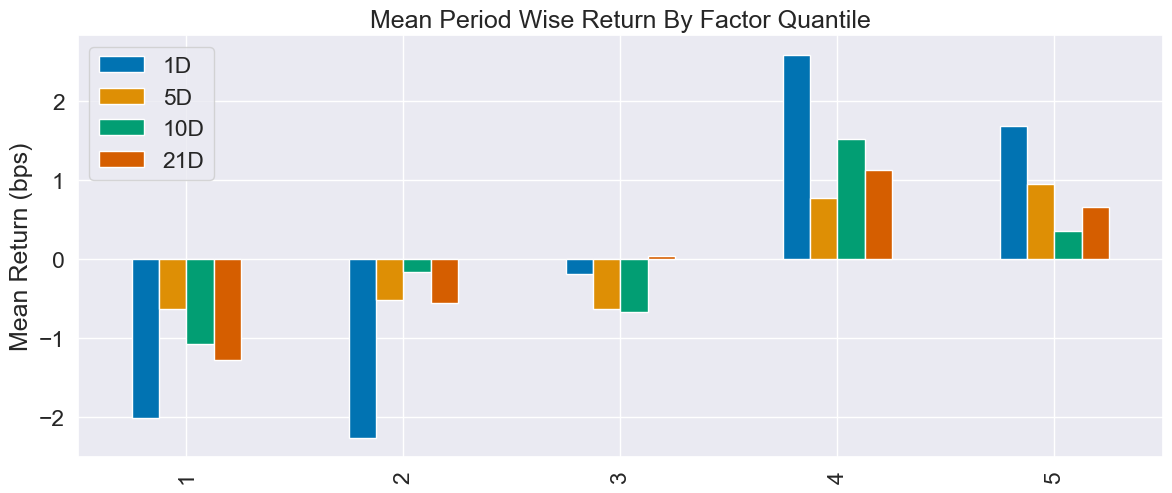
分析：

预测力：跟普通线性回归几乎打平，IC 同样“刚踩线”（0.019→0.021），t-stat 也没飞起来。

赚钱力：1D 对冲 spread 3.7 bps，跟 LR 一样“薄如纸”，扣完双边成本只剩 1 bps 左右。

稳定性：Rank 自相关更高（0.82），换手略低一点，说明岭回归“平滑”后，因子排名短期更耐操，但长周期照样衰减。

总结：岭回归只是“把 LR 的毛刺磨平”，没长出新增信息；成本端省 1 bps，收益端零提升，可留作候选

四、Lasso Regression 套索回归

代码，类似地：

best_lasso_alpha = get_best_alpha(lasso_scores)
lasso_predictions = lasso_predictions[lasso_predictions.alpha==best_lasso_alpha].drop('alpha', axis=1)

lasso_factor = get_factor(lasso_predictions.predicted.swaplevel())
lasso_factor.head()

lasso_factor_data = get_clean_factor_and_forward_returns(factor=lasso_factor,
                                                      prices=trade_prices,
                                                      quantiles=5,
                                                      periods=(1, 5, 10, 21))
lasso_factor_data.info()

create_summary_tear_sheet(lasso_factor_data);

结果：

Dropped 0.0% entries from factor data: 0.0% in forward returns computation and 0.0% in binning phase (set max_loss=0 to see potentially suppressed Exceptions).
max_loss is 35.0%, not exceeded: OK!
<class 'pandas.core.frame.DataFrame'>
MultiIndex: 73812 entries, (Timestamp('2014-12-09 00:00:00+0000', tz='UTC'), 'AAL') to (Timestamp('2017-11-29 00:00:00+0000', tz='UTC'), 'XOM')
Data columns (total 6 columns):
 #   Column           Non-Null Count  Dtype  
---  ------           --------------  -----  
 0   1D               73812 non-null  float64
 1   5D               73812 non-null  float64
 2   10D              73812 non-null  float64
 3   21D              73812 non-null  float64
 4   factor           73812 non-null  float64
 5   factor_quantile  73812 non-null  int64  
dtypes: float64(5), int64(1)
memory usage: 3.7+ MB

Quantiles Statistics

	min	max	mean	std	count	count %
factor_quantile
1	-0.043925	0.010653	-0.003470	0.004004	14982	20.297513
2	-0.013494	0.012950	-0.001383	0.003265	14666	19.869398
3	-0.011373	0.014600	-0.000327	0.003284	14516	19.666179
4	-0.010174	0.016758	0.000706	0.003431	14666	19.869398
5	-0.008641	0.035891	0.002654	0.004164	14982	20.297513

Returns Analysis

	1D	5D	10D	21D
Ann. alpha	0.048	0.017	0.019	0.020
beta	-0.017	-0.068	-0.058	0.041
Mean Period Wise Return Top Quantile (bps)	1.842	1.016	0.514	0.778
Mean Period Wise Return Bottom Quantile (bps)	-1.847	-0.613	-0.910	-1.259
Mean Period Wise Spread (bps)	3.689	1.652	1.433	2.028

Information Analysis

	1D	5D	10D	21D
IC Mean	0.019	0.017	0.019	0.023
IC Std.	0.178	0.165	0.172	0.156
Risk-Adjusted IC	0.107	0.100	0.111	0.148
t-stat(IC)	2.940	2.744	3.053	4.045
p-value(IC)	0.003	0.006	0.002	0.000
IC Skew	-0.093	0.031	-0.158	-0.142
IC Kurtosis	-0.212	-0.053	-0.107	-0.231

Turnover Analysis

	1D	5D	10D	21D
Quantile 1 Mean Turnover	0.300	0.527	0.630	0.747
Quantile 2 Mean Turnover	0.516	0.705	0.758	0.797
Quantile 3 Mean Turnover	0.560	0.739	0.773	0.807
Quantile 4 Mean Turnover	0.515	0.704	0.756	0.789
Quantile 5 Mean Turnover	0.302	0.530	0.637	0.741