python使用opencv对图像的基本操作(4)

19.调整图片强度

19.1.调整强度

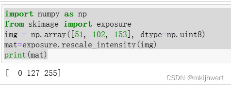
import numpy as np
from skimage import exposure
img = np.array([51, 102, 153], dtype=np.uint8)
mat=exposure.rescale_intensity(img)
print(mat)

注：skimage.exposure.rescale_intensity函数来调整img数组的亮度范围。这个函数会将图像的亮度范围从当前范围调整为0到255，如果图像的亮度范围已经在这个范围内，则不会进行任何调整。调整后的数组被存储在变量mat中。
运行结果：

19.2.使用uint8转float调整增强度

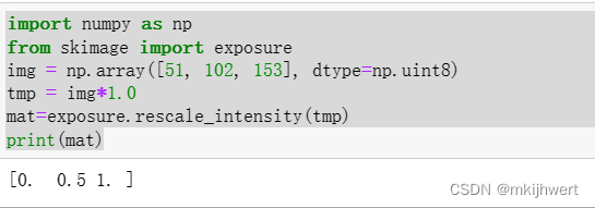
import numpy as np
from skimage import exposure
img = np.array([51, 102, 153], dtype=np.uint8)
tmp = img*1.0
mat=exposure.rescale_intensity(tmp)
print(mat)

注：tmp = img*1.0：这行代码创建了一个新的数组tmp，被转换为浮点数类型，这是因为exposure.rescale_intensity函数期望输入为浮点数类型。
运行结果：

20.绘制直方图

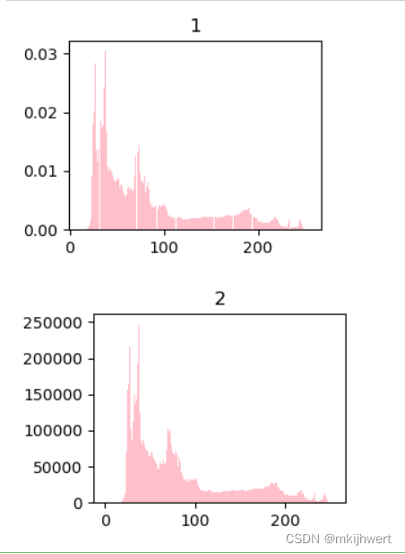
20.1.将原图和归一化后的图片进行对比

from skimage import io
import matplotlib.pyplot as plt
img=io.imread('ww.jpg')
img1=io.imread("D:\ww1.jpg")

plt.subplot(221)
plt.title('1')
arr=img.flatten()
n, bins, patches = plt.hist(arr, bins=256, density=True,edgecolor='None',facecolor='pink')
plt.show()


plt.subplot(221)
plt.title('2')
arr=img1.flatten()
n, bins, patches = plt.hist(arr, bins=256, density=0,edgecolor='None',facecolor='pink')
plt.show()

注：
hist的参数非常多，但常用的就这六个，只有第一个是必须的，后面四个可选。
arr: 需要计算直方图的一维数组。
bins: 直方图的柱数，可选项，默认为10。
normed: 是否将得到的直方图向量归一化，默认为0。
facecolor: 直方图颜色。
edgecolor: 直方图边框颜色。
alpha: 透明度。
histtype: 直方图类型，‘bar’, ‘barstacked’, ‘step’, ‘stepfilled’。
n: 直方图向量，是否归一化由参数normed设定。
bins: 返回各个bin的区间范围。
patches: 返回每个bin里面包含的数据，是一个list。
运行结果：

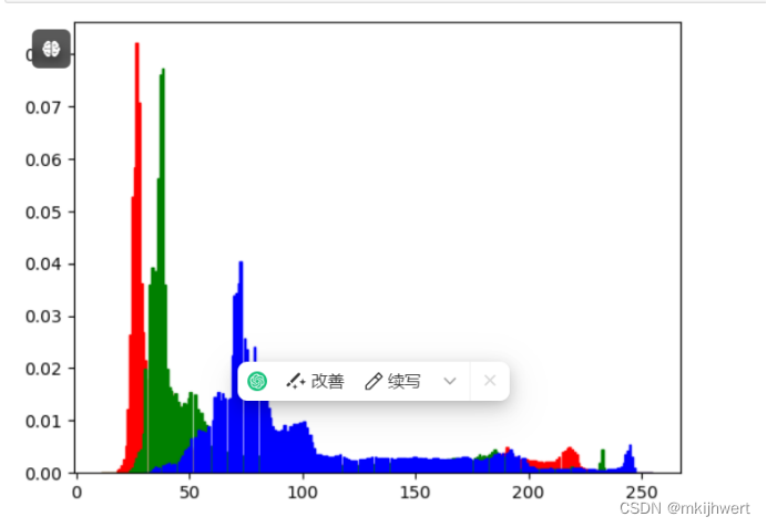
20.2绘制三通道的直方图

from skimage import io
import matplotlib.pyplot as plt
img=io.imread('ww.jpg')
ar=img[:,:,0].flatten()
plt.hist(ar, bins=256, density=1,facecolor='r',edgecolor='r')

ar=img[:,:,1].flatten()
plt.hist(ar, bins=256, density=1,facecolor='g',edgecolor='g')

ar=img[:,:,2].flatten()
plt.hist(ar, bins=256, density=1,facecolor='b',edgecolor='b')
plt.show()
#hold=1表示可以叠加

注：hold=1表示可以叠加。
运行结果：

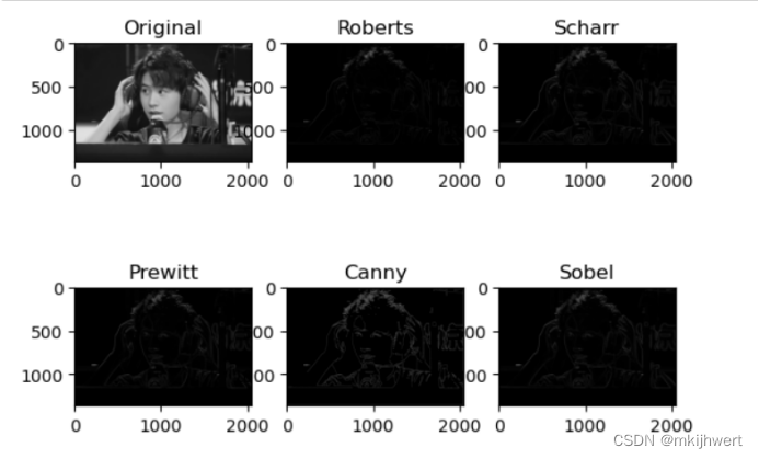
21.使用微分算子对图像进行滤波

21.1.sobel算子/roberts算子/scharr算子/canny算子/prewitt算子

from skimage import io, filters, color,feature
import matplotlib.pyplot as plt

# 读取图片
img = io.imread('ww.jpg')

# 转换图片到灰度
img_gray = color.rgb2gray(img)

# 创建子图
plt.subplot(2, 3, 1)
plt.title('Original')
plt.imshow(img_gray, cmap=plt.cm.gray)

plt.subplot(2, 3, 2)
plt.title('Roberts')  #roberts算子
edges1 = filters.roberts(img_gray)
plt.imshow(edges1, cmap=plt.cm.gray)

plt.subplot(2, 3, 3)
plt.title('Scharr')   #scharr算子
edges2 = filters.scharr(img_gray)
plt.imshow(edges2, cmap=plt.cm.gray)

plt.subplot(2, 3, 4)
plt.title('Prewitt')   #prewitt算子
edges3 = filters.prewitt(img_gray)
plt.imshow(edges3, cmap=plt.cm.gray)

plt.subplot(2, 3, 5)
plt.title('Canny')    #canny算子
edges4 = feature.canny(img_gray)
plt.imshow(edges4, cmap=plt.cm.gray)

plt.subplot(2, 3, 6)
plt.title('Sobel')    # sobel算子
edges5 = filters.sobel(img_gray)
plt.imshow(edges5, cmap=plt.cm.gray)

# 显示所有子图
plt.show()

注：sobel算子可用来检测边缘，canny算子也是用于提取边缘特征，但它不是放在filters模块，而是放在feature模块。
运行结果：

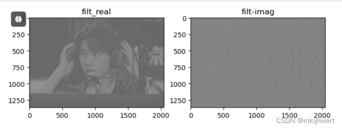
21.2.使用Gabor滤波器对图像进行处理

from skimage import data,filters,color
import matplotlib.pyplot as plt
img = io.imread('ww.jpg')
img_gray = color.rgb2gray(img)
filt_real, filt_img = filters.gabor(img_gray,frequency=0.6)   
 
plt.figure('gabor',figsize=(8,8))
 
plt.subplot(121)
plt.title('filt_real')
plt.imshow(filt_real,plt.cm.gray)  

plt.subplot(122)
plt.title('filt-imag')
plt.imshow(filt_img,plt.cm.gray)
 
plt.show()

注：filters模块包含了一系列用于图像滤波的函数，frequency=0.6参数指定了滤波器的频率，即它检测的纹理尺度的粗细。
运行结果：

22.在图片上绘制图形

22.1.画线条

#line划线
from skimage import draw
import matplotlib.pyplot as plt
img = io.imread('ww.jpg')
rr, cc = draw.line(10, 500, 400, 600)
draw.set_color(img,[rr, cc],[202,235,216])
plt.imshow(img,plt.cm.gray)

注：draw模块包含了一系列用于在图像上绘制形状和线条的函数。
运行结果：

22.2.绘制圆形

#disk圆形
from skimage import io
import matplotlib.pyplot as plt
img = io.imread('xxz.jpg')
rr, cc=draw.disk((350,350),50)
draw.set_color(img,[rr, cc],[202,235,216])
plt.imshow(img,plt.cm.gray)

运行结果：

22.3.绘制椭圆

#ellipse椭圆
from skimage import io,draw
import matplotlib.pyplot as plt
img = io.imread('ww.jpg')
rr, cc=draw.ellipse(550,820,40,90)
draw.set_color(img,[rr, cc],[255,192,203])
plt.imshow(img,plt.cm.gray)

运行结果：

22.4.绘制多边形

#多边形
from skimage import draw,io
import matplotlib.pyplot as plt
import numpy as np
img = io.imread('ww.jpg')
Y = np.array([200, 200, 360, 500, 500, 360])
X = np.array([300, 400, 450, 400, 300, 250])
rr, cc=draw.polygon(Y,X)
draw.set_color(img,[rr,cc],[202,235,216])
plt.imshow(img,plt.cm.gray)

注：Y = np.array([200, 200, 360, 500, 500, 360])：这行代码创建了一个包含六个元素的数组Y，这些元素代表了多边形顶点的y坐标。
X = np.array([300, 400, 450, 400, 300, 250])：这行代码创建了一个包含六个元素的数组X，这些元素代表了多边形顶点的x坐标。
运行结果：

22.5.绘制空心圆

#perimeter是绘制空心圆
from skimage import draw,io
import matplotlib.pyplot as plt
img = io.imread('ww.jpg')
rr, cc=draw.circle_perimeter(350,350,300)
draw.set_color(img,[rr, cc],[202,235,216])
plt.imshow(img,plt.cm.gray)

运行结果：

23.对图像进行角度旋转、水平、垂直镜像操作

import matplotlib.pyplot as plt 
import matplotlib.image as mpimg 
import numpy as np

img = mpimg.imread('ww.jpg')
#使用numpy.rot90函数将img图像旋转90度。
rotated_img = np.rot90(img)
#使用numpy.fliplr函数将img图像沿水平轴翻转。
flipped_img_horizontal = np.fliplr(img)
flipped_img_vertical = np.flipud(img)  # 定义垂直翻转的图像

plt.subplot(2, 2, 1) 
plt.imshow(img) 
plt.title('Original Image')
plt.axis('off')

plt.subplot(2, 2, 2) 
plt.imshow(rotated_img) 
plt.title('Rotated Image')
plt.axis('off')

plt.subplot(2, 2, 3) 
plt.imshow(flipped_img_horizontal) 
plt.title('Flipped Horizontal Image')
plt.axis('off')

plt.subplot(2, 2, 4) 
plt.imshow(flipped_img_vertical) 
plt.title('Flipped Vertical Image')
plt.axis('off')

plt.show()

注：flipped_img_vertical = np.flipud(img)：这行代码使用numpy.flipud函数将img图像沿垂直轴翻转。翻转后的图像被存储在变量flipped_img_vertical中。
运行结果：