Python基础（十） Numpy详细教程_python的numpy教程csdn

x5[0, 0] = 0
x5

array([[ 0, 14],
       [ 8, 12]])

x4

array([[ 0, 14,  7,  2],
       [ 8, 12,  9,  3],
       [19,  0, 10,  7]])

修改切片的安全方式：copy

x4 = np.random.randint(20, size=(3,4)) 
x4

array([[18, 14, 10, 12],
       [10, 16,  7, 19],
       [ 3, 16,  3, 12]])

x6 = x4[:2, :2].copy()
x6

array([[18, 14],
       [10, 16]])

x6[0, 0] = 0
x6

array([[ 0, 14],
       [10, 16]])

x4

array([[18, 14, 10, 12],
       [10, 16,  7, 19],
       [ 3, 16,  3, 12]])

10.3.4 数组的变形

x5 = np.random.randint(0, 10, (12,))
x5

array([5, 0, 1, 3, 2, 6, 3, 8, 7, 5, 2, 5])

x5.shape

(12,)

x6 = x5.reshape(3, 4)
x6

array([[9, 8, 5, 9],
       [2, 6, 2, 9],
       [4, 5, 1, 7]])

注意：reshape返回的是视图，而非副本

x6[0, 0] = 0
x5

array([0, 8, 5, 9, 2, 6, 2, 9, 4, 5, 1, 7])

一维向量转行向量

x7 = x5.reshape(1, x5.shape[0])    
x7

array([[0, 8, 5, 9, 2, 6, 2, 9, 4, 5, 1, 7]])

x8 = x5[np.newaxis, :]
x8

array([[0, 8, 5, 9, 2, 6, 2, 9, 4, 5, 1, 7]])

一维向量转列向量

x7 = x5.reshape(x5.shape[0], 1)    
x7

array([[0],
       [8],
       [5],
       [9],
       [2],
       [6],
       [2],
       [9],
       [4],
       [5],
       [1],
       [7]])

x8 = x5[:, np.newaxis]
x8

array([[0],
       [8],
       [5],
       [9],
       [2],
       [6],
       [2],
       [9],
       [4],
       [5],
       [1],
       [7]])

多维向量转一维向量

x6 = np.random.randint(0, 10, (3, 4))
x6

array([[3, 7, 6, 4],
       [4, 5, 6, 3],
       [7, 6, 2, 3]])

flatten返回的是副本

x9 = x6.flatten()
x9

array([3, 7, 6, 4, 4, 5, 6, 3, 7, 6, 2, 3])

x9[0]=0
x6

array([[3, 7, 6, 4],
       [4, 5, 6, 3],
       [7, 6, 2, 3]])

ravel返回的是视图

x10 = x6.ravel()
x10

array([3, 7, 6, 4, 4, 5, 6, 3, 7, 6, 2, 3])

x10[0]=0
x6

array([[0, 7, 6, 4],
       [4, 5, 6, 3],
       [7, 6, 2, 3]])

reshape返回的是视图

x11 = x6.reshape(-1)
x11

array([0, 7, 6, 4, 4, 5, 6, 3, 7, 6, 2, 3])

x11[0]=10
x6

array([[10,  7,  6,  4],
       [ 4,  5,  6,  3],
       [ 7,  6,  2,  3]])

10.3.5 数组的拼接

x1 = np.array([[1, 2, 3],
              [4, 5, 6]])
x2 = np.array([[7, 8, 9],
              [0, 1, 2]])

1、水平拼接——非视图

• hstack()
• c_

x3 = np.hstack([x1, x2])
x3

array([[1, 2, 3, 7, 8, 9],
       [4, 5, 6, 0, 1, 2]])

x3[0][0] = 0
x1

array([[1, 2, 3],
       [4, 5, 6]])

x4 = np.c_[x1, x2]
x4

array([[1, 2, 3, 7, 8, 9],
       [4, 5, 6, 0, 1, 2]])

x4[0][0] = 0
x1

array([[1, 2, 3],
       [4, 5, 6]])

2、垂直拼接——非视图

• vstack()
• r_

x1 = np.array([[1, 2, 3],
              [4, 5, 6]])
x2 = np.array([[7, 8, 9],
              [0, 1, 2]])

x5 = np.vstack([x1, x2])
x5

array([[1, 2, 3],
       [4, 5, 6],
       [7, 8, 9],
       [0, 1, 2]])

x6 = np.r_[x1, x2]
x6

array([[1, 2, 3],
       [4, 5, 6],
       [7, 8, 9],
       [0, 1, 2]])

10.3.6 数组的分裂

1、split的用法

x6 = np.arange(10)
x6

array([0, 1, 2, 3, 4, 5, 6, 7, 8, 9])

x1, x2, x3 = np.split(x6, [2, 7]) #分裂点的位置，前向（从0开始）
print(x1, x2, x3)

[0 1] [2 3 4 5 6] [7 8 9]

2、hsplit的用法

x7 = np.arange(1, 26).reshape(5, 5)
x7

array([[ 1,  2,  3,  4,  5],
       [ 6,  7,  8,  9, 10],
       [11, 12, 13, 14, 15],
       [16, 17, 18, 19, 20],
       [21, 22, 23, 24, 25]])

left, middle, right = np.hsplit(x7, [2,4])
print("left:\n", left)            # 第0~1列
print("middle:\n", middle)        # 第2~3列
print("right:\n", right)          # 第4列

left:
 [[ 1  2]
 [ 6  7]
 [11 12]
 [16 17]
 [21 22]]
middle:
 [[ 3  4]
 [ 8  9]
 [13 14]
 [18 19]
 [23 24]]
right:
 [[ 5]
 [10]
 [15]
 [20]
 [25]]

3、vsplit的用法

x7 = np.arange(1, 26).reshape(5, 5)
x7

array([[ 1,  2,  3,  4,  5],
       [ 6,  7,  8,  9, 10],
       [11, 12, 13, 14, 15],
       [16, 17, 18, 19, 20],
       [21, 22, 23, 24, 25]])

upper, middle, lower = np.vsplit(x7, [2,4])
print("upper:\n", upper)         # 第0~1行
print("middle:\n", middle)       # 第2~3行
print("lower:\n", lower)         # 第4行

upper:
 [[ 1  2  3  4  5]
 [ 6  7  8  9 10]]
middle:
 [[11 12 13 14 15]
 [16 17 18 19 20]]
lower:
 [[21 22 23 24 25]]

10.4 Numpy四大运算

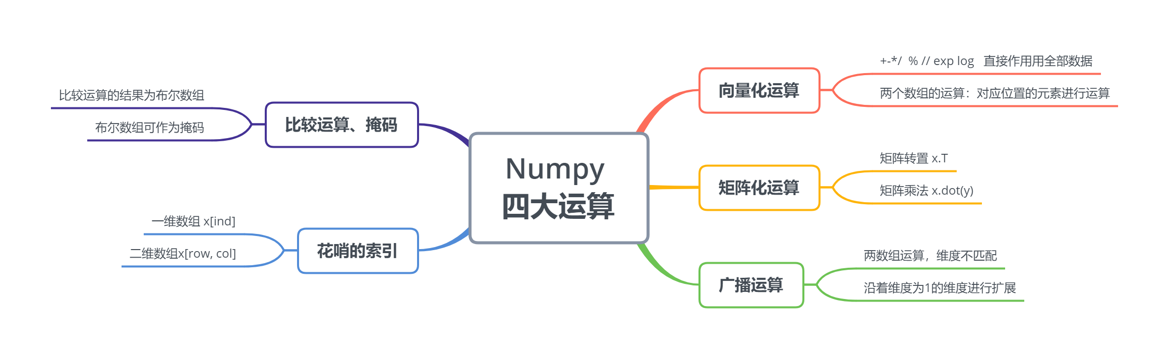
10.4.1 向量化运算

1、与数字的加减乘除等 可见整体进行了向量化的运算

x1 = np.arange(1,6)
x1

array([1, 2, 3, 4, 5])

print("x1+5", x1+5)
print("x1-5", x1-5)
print("x1\*5", x1\*5)
print("x1/5", x1/5)

x1+5 [ 6  7  8  9 10]
x1-5 [-4 -3 -2 -1  0]
x1*5 [ 5 10 15 20 25]
x1/5 [0.2 0.4 0.6 0.8 1. ]

print("-x1", -x1)
print("x1\*\*2", x1\*\*2)
print("x1//2", x1//2)
print("x1%2", x1%2)

-x1 [-1 -2 -3 -4 -5]
x1**2 [ 1  4  9 16 25]
x1//2 [0 1 1 2 2]
x1%2 [1 0 1 0 1]

2、绝对值、三角函数、指数、对数

（1）绝对值

x2 = np.array([1, -1, 2, -2, 0])
x2

array([ 1, -1,  2, -2,  0])

abs(x2)

array([1, 1, 2, 2, 0])

np.abs(x2)

array([1, 1, 2, 2, 0])

（2）三角函数

theta = np.linspace(0, np.pi, 3)
theta

array([0.        , 1.57079633, 3.14159265])

print("sin(theta)", np.sin(theta))
print("con(theta)", np.cos(theta))
print("tan(theta)", np.tan(theta))

sin(theta) [0.0000000e+00 1.0000000e+00 1.2246468e-16]
con(theta) [ 1.000000e+00  6.123234e-17 -1.000000e+00]
tan(theta) [ 0.00000000e+00  1.63312394e+16 -1.22464680e-16]

x = [1, 0 ,-1]
print("arcsin(x)", np.arcsin(x))
print("arccon(x)", np.arccos(x))
print("arctan(x)", np.arctan(x))

arcsin(x) [ 1.57079633  0.         -1.57079633]
arccon(x) [0.         1.57079633 3.14159265]
arctan(x) [ 0.78539816  0.         -0.78539816]

（3）指数运算

x = np.arange(3)
x

array([0, 1, 2])

np.exp(x)

array([1.        , 2.71828183, 7.3890561 ])

（4）对数运算

x = np.array([1, 2, 4, 8 ,10])
print("ln(x)", np.log(x))
print("log2(x)", np.log2(x))
print("log10(x)", np.log10(x))

ln(x) [0.         0.69314718 1.38629436 2.07944154 2.30258509]
log2(x) [0.         1.         2.         3.         3.32192809]
log10(x) [0.         0.30103    0.60205999 0.90308999 1.        ]

3、两个数组的运算

x1 = np.arange(1,6)
x1

array([1, 2, 3, 4, 5])

x2 = np.arange(6,11)
x2

array([ 6,  7,  8,  9, 10])

print("x1+x2:", x1+x2)
print("x1-x2:", x1-x2)
print("x1\*x2:", x1\*x2)
print("x1/x2:", x1/x2)

x1+x2: [ 7  9 11 13 15]
x1-x2: [-5 -5 -5 -5 -5]
x1*x2: [ 6 14 24 36 50]
x1/x2: [0.16666667 0.28571429 0.375      0.44444444 0.5       ]

10.4.2 矩阵运算

x = np.arange(9).reshape(3, 3)
x

array([[0, 1, 2],
       [3, 4, 5],
       [6, 7, 8]])

• 矩阵的转置

y = x.T
y

array([[0, 3, 6],
       [1, 4, 7],
       [2, 5, 8]])

• 矩阵乘法

x = np.array([[1, 0],
             [1, 1]])
y = np.array([[0, 1],
             [1, 1]])

x.dot(y)

array([[0, 1],
       [1, 2]])

np.dot(x, y)

array([[0, 1],
       [1, 2]])

y.dot(x)

array([[1, 1],
       [2, 1]])

np.dot(y, x)

array([[1, 1],
       [2, 1]])

注意跟x*y的区别，x*y只是对应位置相乘

x\*y

array([[0, 0],
       [1, 1]])

10.4.3 广播运算

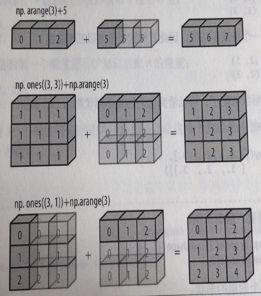
x = np.arange(3).reshape(1, 3)
x

array([[0, 1, 2]])

x+5

array([[5, 6, 7]])

规则

如果两个数组的形状在维度上不匹配

那么数组的形式会沿着维度为1的维度进行扩展以匹配另一个数组的形状。

x1 = np.ones((3,3))
x1

array([[1., 1., 1.],
       [1., 1., 1.],
       [1., 1., 1.]])

x2 = np.arange(3).reshape(1, 3)
x2

array([[0, 1, 2]])

x1+x2

array([[1., 2., 3.],
       [1., 2., 3.],
       [1., 2., 3.]])

x3 = np.logspace(1, 10, 10, base=2).reshape(2, 5)
x3

array([[   2.,    4.,    8.,   16.,   32.],
       [  64.,  128.,  256.,  512., 1024.]])

x4 = np.array([[1, 2, 4, 8, 16]])
x4

array([[ 1,  2,  4,  8, 16]])

x3/x4

array([[ 2.,  2.,  2.,  2.,  2.],
       [64., 64., 64., 64., 64.]])

x5 = np.arange(3).reshape(3, 1)
x5

array([[0],
       [1],
       [2]])

x6 = np.arange(3).reshape(1, 3)
x6

array([[0, 1, 2]])

x5+x6

array([[0, 1, 2],
       [1, 2, 3],
       [2, 3, 4]])

10.4.4 比较运算和掩码

1、比较运算

x1 = np.random.randint(100, size=(10,10))
x1

array([[37, 44, 58, 79,  1, 24, 85, 90, 27, 56],
       [74, 68, 88, 27, 46, 34, 92,  1, 35, 45],
       [84, 80, 83, 72, 98, 15,  4, 77, 14, 98],
       [19, 85, 98, 32, 47, 50, 73,  3, 24,  2],
       [ 5, 28, 26, 31, 48, 43, 72, 73, 53, 64],
       [81, 87, 56, 59, 24, 42, 84, 34, 97, 65],
       [74,  9, 41, 54, 78, 62, 53, 49,  8, 70],
       [63, 44, 33, 35, 26, 83,  7, 14, 65, 84],
       [57, 10, 62,  8, 74, 47, 90, 25, 78, 48],
       [36, 31, 45, 39, 66, 82, 42, 25, 33, 84]])

x1 > 50

array([[False, False,  True,  True, False, False,  True,  True, False,
         True],
       [ True,  True,  True, False, False, False,  True, False, False,
        False],
       [ True,  True,  True,  True,  True, False, False,  True, False,
         True],
       [False,  True,  True, False, False, False,  True, False, False,
        False],
       [False, False, False, False, False, False,  True,  True,  True,
         True],
       [ True,  True,  True,  True, False, False,  True, False,  True,
         True],
       [ True, False, False,  True,  True,  True,  True, False, False,
         True],
       [ True, False, False, False, False,  True, False, False,  True,
         True],
       [ True, False,  True, False,  True, False,  True, False,  True,
        False],
       [False, False, False, False,  True,  True, False, False, False,
         True]])

2、操作布尔数组

x2 = np.random.randint(10, size=(3, 4))
x2

array([[1, 4, 2, 9],
       [8, 8, 2, 4],
       [9, 5, 3, 6]])

print(x2 > 5)
np.sum(x2 > 5)

[[False False False  True]
 [ True  True False False]
 [ True False False  True]]

5

np.all(x2 > 0)

True

np.any(x2 == 6)

True

np.all(x2 < 9, axis=1)   # 按行进行判断 axis = 1。而如果是按列判断，则axis= 0;

array([False,  True, False])

x2

array([[1, 4, 2, 9],
       [8, 8, 2, 4],
       [9, 5, 3, 6]])

(x2 < 9) & (x2 >5)

array([[False, False, False, False],
       [ True,  True, False, False],
       [False, False, False,  True]])

np.sum((x2 < 9) & (x2 >5))

3

3、将布尔数组作为掩码

x2

array([[1, 4, 2, 9],
       [8, 8, 2, 4],
       [9, 5, 3, 6]])

x2 > 5

array([[False, False, False,  True],
       [ True,  True, False, False],
       [ True, False, False,  True]])

x2[x2 > 5]

array([9, 8, 8, 9, 6])

作为掩码后，相应位置为True的就会被取出来，而相应位置为False的就会忽略

10.4.5 花哨的索引

1、一维数组

x = np.random.randint(100, size=10)
x

array([43, 69, 67,  9, 11, 27, 55, 93, 23, 82])

注意：结果的形状与索引数组ind一致

ind = [2, 6, 9]
x[ind]

array([67, 55, 82])

ind = np.array([[1, 0],
               [2, 3]])
x[ind]

array([[69, 43],
       [67,  9]])

2、多维数组

x = np.arange(12).reshape(3, 4)
x

array([[ 0,  1,  2,  3],
       [ 4,  5,  6,  7],
       [ 8,  9, 10, 11]])

row = np.array([0, 1, 2])
col = np.array([1, 3, 0])
x[row, col]               # x(0, 1) x(1, 3) x(2, 0)

array([1, 7, 8])

row[:, np.newaxis]       # 列向量

array([[0],
       [1],
       [2]])

x[row[:, np.newaxis], col]    # 广播机制

array([[ 1,  3,  0],
       [ 5,  7,  4],
       [ 9, 11,  8]])

10.5 其他Numpy通用函数

10.5.1 数值排序

x = np.random.randint(20, 50, size=10)
x

array([48, 27, 44, 24, 34, 21, 24, 30, 34, 46])

• 产生新的排序数组

np.sort(x)

array([21, 24, 24, 27, 30, 34, 34, 44, 46, 48])

x

array([48, 27, 44, 24, 34, 21, 24, 30, 34, 46])

• 替换原数组

x.sort()
x

array([21, 24, 24, 27, 30, 34, 34, 44, 46, 48])

• 获得排序索引

x = np.random.randint(20, 50, size=10)
x

array([27, 36, 35, 28, 34, 20, 21, 49, 48, 30])

i = np.argsort(x)
i

array([5, 6, 0, 3, 9, 4, 2, 1, 8, 7], dtype=int64)

10.5.2 最大最小值

x = np.random.randint(20, 50, size=10)
x

array([48, 31, 30, 44, 48, 33, 44, 48, 39, 35])

print("max:", np.max(x))
print("min:", np.min(x))

max: 48
min: 30

print("max\_index:", np.argmax(x))
print("min\_index:", np.argmin(x))

max_index: 0
min_index: 2

10.5.3 数值求和、求积

x = np.arange(1,6)
x

array([1, 2, 3, 4, 5])

x.sum()

15

np.sum(x)

15

x1 = np.arange(6).reshape(2,3)
x1

array([[0, 1, 2],
       [3, 4, 5]])

• 按行求和

np.sum(x1, axis=1)

array([ 3, 12])

• 按列求和

np.sum(x1, axis=0)

array([3, 5, 7])

一、Python所有方向的学习路线

Python所有方向路线就是把Python常用的技术点做整理，形成各个领域的知识点汇总，它的用处就在于，你可以按照上面的知识点去找对应的学习资源，保证自己学得较为全面。

二、学习软件

工欲善其事必先利其器。学习Python常用的开发软件都在这里了，给大家节省了很多时间。

三、入门学习视频

我们在看视频学习的时候，不能光动眼动脑不动手，比较科学的学习方法是在理解之后运用它们，这时候练手项目就很适合了。

网上学习资料一大堆，但如果学到的知识不成体系，遇到问题时只是浅尝辄止，不再深入研究，那么很难做到真正的技术提升。

需要这份系统化学习资料的朋友，可以戳这里无偿获取

一个人可以走的很快，但一群人才能走的更远！不论你是正从事IT行业的老鸟或是对IT行业感兴趣的新人，都欢迎加入我们的的圈子（技术交流、学习资源、职场吐槽、大厂内推、面试辅导），让我们一起学习成长！