


既有适合小白学习的零基础资料,也有适合3年以上经验的小伙伴深入学习提升的进阶课程,涵盖了95%以上大数据知识点,真正体系化!
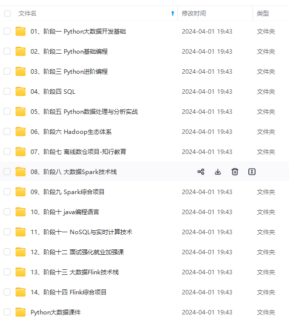
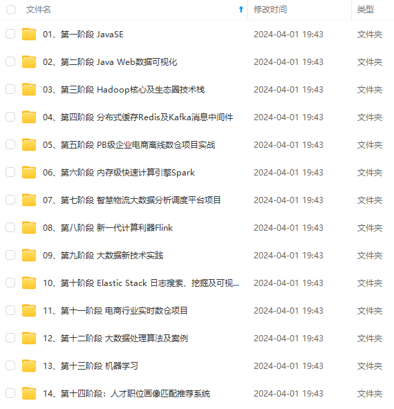
由于文件比较多,这里只是将部分目录截图出来,全套包含大厂面经、学习笔记、源码讲义、实战项目、大纲路线、讲解视频,并且后续会持续更新
## 1.数据收集和加载


我们将使用kaggle提供的数据集:[数据集](https://bbs.csdn.net/topics/618545628)


该数据集 包含一组带有标记的短信文本,这些消息被归类为**正常短信**和**垃圾短信。** 每行包含一条消息。每行由两列组成:v1 带有标签,(spam 或 ham),v2 是文本内容。
df=pd.read_csv(‘/content/spam/spam.csv’,encoding=‘latin-1’)#这里encoding需要指定为latin-1
查看一下数据基本情况
df.head()
|  | v1 | v2 | Unnamed: 2 | Unnamed: 3 | Unnamed: 4 |
| --- | --- | --- | --- | --- | --- |
| 0 | ham | Go until jurong point, crazy.. Available only ... | NaN | NaN | NaN |
| 1 | ham | Ok lar... Joking wif u oni... | NaN | NaN | NaN |
| 2 | spam | Free entry in 2 a wkly comp to win FA Cup fina... | NaN | NaN | NaN |
| 3 | ham | U dun say so early hor... U c already then say... | NaN | NaN | NaN |
| 4 | ham | Nah I don't think he goes to usf, he lives aro... | NaN | NaN | NaN |


该数据包含一组带有标记的短信数据,其中:


>
> * v1表示短信标签,**ham表示正常信息,spam表示垃圾信息**
> * v2是短信的内容
>
>
>
#去除不需要的列
df=df.iloc[:,:2]
#重命名列
df=df.rename(columns={“v1”:“label”,“v2”:“message”})
df.head()
|  | label | message |
| --- | --- | --- |
| 0 | ham | Go until jurong point, crazy.. Available only ... |
| 1 | ham | Ok lar... Joking wif u oni... |
| 2 | spam | Free entry in 2 a wkly comp to win FA Cup fina... |
| 3 | ham | U dun say so early hor... U c already then say... |
| 4 | ham | Nah I don't think he goes to usf, he lives aro... |
将lable进行one-hot编码,其中0:ham,1:spam
from sklearn.preprocessing import LabelEncoder
encoder = LabelEncoder()
df[‘label’]=encoder.fit_transform(df[‘label’])
df[‘label’].value_counts()
0 4825
1 747
Name: label, dtype: int64
可以看出一共有747个垃圾短信
查看缺失值
df.isnull().sum()
数据没有缺失值
label 0
message 0
dtype: int64
## 2.探索性数据分析(EDA)


通过可视化分析来更好的理解数据
import matplotlib.pyplot as plt
plt.style.use(‘ggplot’)
plt.figure(figsize=(9,4))
plt.subplot(1,2,1)
plt.pie(df[‘label’].value_counts(),labels=[‘not spam’,‘spam’],autopct=“%0.2f”)
plt.subplot(1,2,2)
sns.barplot(x=df[‘label’].value_counts().index,y=df[‘label’].value_counts(),data=df)
plt.show()

在特征工程部分,我简单创建了一些单独的特征来提取信息
* 字符数
* 单词数
* 句子数
#1.字符数
df[‘char’]=df[‘message’].apply(len)
nltk.download(‘punkt’)
[nltk_data] Downloading package punkt to /root/nltk_data…
[nltk_data] Unzipping tokenizers/punkt.zip.
True
#2.单词数,这里我们首先要对其进行分词处理,使用nltk
#分词处理
df[‘words’]=df[‘message’].apply(lambda x: len(nltk.word_tokenize(x)))
3.句子数
df[‘sen’]=df[‘message’].apply(lambda x: len(nltk.sent_tokenize(x)))
df.head()
|  | label | message | char | words | sen |
| --- | --- | --- | --- | --- | --- |
| 0 | 0 | Go until jurong point, crazy.. Available only ... | 111 | 24 | 2 |
| 1 | 0 | Ok lar... Joking wif u oni... | 29 | 8 | 2 |
| 2 | 1 | Free entry in 2 a wkly comp to win FA Cup fina... | 155 | 37 | 2 |
| 3 | 0 | U dun say so early hor... U c already then say... | 49 | 13 | 1 |
| 4 | 0 | Nah I don't think he goes to usf, he lives aro... | 61 | 15 | 1 |


**描述性统计**
描述性统计
df.describe()
| index | label | char | words | sen |
| --- | --- | --- | --- | --- |
| count | 5572.0 | 5572.0 | 5572.0 | 5572.0 |
| mean | 0.13406317300789664 | 80.11880832735105 | 18.69562096195262 | 1.9707465900933239 |
| std | 0.34075075489776974 | 59.6908407765033 | 13.742586801744975 | 1.4177777134026657 |
| min | 0.0 | 2.0 | 1.0 | 1.0 |
| 25% | 0.0 | 36.0 | 9.0 | 1.0 |
| 50% | 0.0 | 61.0 | 15.0 | 1.0 |
| 75% | 0.0 | 121.0 | 27.0 | 2.0 |
| max | 1.0 | 910.0 | 220.0 | 28.0 |


下面我们通过可视化比较一下不同短信在这些数字特征上的分布情况
字符数比较
plt.figure(figsize=(12,6))
sns.histplot(df[df[‘label’]==0][‘char’],color=‘red’)#正常短信
sns.histplot(df[df[‘label’]==1][‘char’],color = ‘blue’)#垃圾短信
<matplotlib.axes._subplots.AxesSubplot at 0x7fce63763dd0>

比较
plt.figure(figsize=(12,6))
sns.histplot(df[df[‘label’]==0][‘words’],color=‘red’)#正常短信
sns.histplot(df[df[‘label’]==1][‘words’],color = ‘blue’)#垃圾短信
<matplotlib.axes._subplots.AxesSubplot at 0x7fce63f4bed0>

sns.pairplot(df,hue=‘label’)

#删除数据集中存在的一些异常值
i=df[df[‘char’]>500].index
df.drop(i,axis=0,inplace=True)
df=df.reset_index()
df.drop(“index”,inplace=True,axis=1)
#相关系数矩阵
sns.heatmap(df.corr(),annot=True)
<matplotlib.axes._subplots.AxesSubplot at 0x7fce606d0250>

我们这里看到存在多重共线性,因此,我们不使用所有的列,在这里选择与label相关性最强的char
## 3.数据预处理
对于英文文本数据,我们常用的数据预处理方式如下
* 去除标点符号
* 去除停用词
* 去除专有名词
* 变换成小写
* 分词处理
* 词根、词缀处理
下面我们来看看如何实现这些步骤
nltk.download(‘stopwords’)
[nltk_data] Downloading package stopwords to /root/nltk_data…
[nltk_data] Unzipping corpora/stopwords.zip.
True
首先导入需要使用到的包
from nltk.corpus import stopwords
from nltk.stem import PorterStemmer
from wordcloud import WordCloud
import string,time
标点符号
string.punctuation
‘!"#$%&’()*+,-./:;<=>?@[\]^_`{|}~’
停用词
stopwords.words(‘english’)
### 3.1清洗文本数据


* 去除web链接
* 去除邮件
* 取掉数字


下面使用正则表达式来处理这些数据。
def remove_website_links(text):
no_website_links = text.replace(r"http\S+", “”)#去除网络连接
return no_website_links
def remove_numbers(text):
removed_numbers = text.replace(r’\d+‘,’')#去除数字
return removed_numbers
def remove_emails(text):
no_emails = text.replace(r"\S*@\S*\s?",‘’)#去除邮件
return no_emails
df[‘message’] = df[‘message’].apply(remove_website_links)
df[‘message’] = df[‘message’].apply(remove_numbers)
df[‘message’] = df[‘message’].apply(remove_emails)
df.head()
|  | label | message | char | words | sen |
| --- | --- | --- | --- | --- | --- |
| 0 | 0 | Go until jurong point, crazy.. Available only ... | 111 | 24 | 2 |
| 1 | 0 | Ok lar... Joking wif u oni... | 29 | 8 | 2 |
| 2 | 1 | Free entry in 2 a wkly comp to win FA Cup fina... | 155 | 37 | 2 |
| 3 | 0 | U dun say so early hor... U c already then say... | 49 | 13 | 1 |
| 4 | 0 | Nah I don't think he goes to usf, he lives aro... | 61 | 15 | 1 |


### 3.2 文本特征转换
def message_transform(text):
text = text.lower()#转换为小写
text = nltk.word_tokenize(text)#分词处理
去除停用词和标点
y = []#创建一个空列表
for word in text:
stopwords_punc = stopwords.words(‘english’)+list(string.punctuation)#存放停用词和标点
if word.isalnum()==True and word not in stopwords_punc:
y.append(word)
词根变换
message=y[:]
y.clear()
for i in message:
ps=PorterStemmer()
y.append(ps.stem(i))
return " ".join(y)#返回字符串形式
df[‘message’] = df[‘message’].apply(message_transform)
df[‘num_words_transform’]=df[‘message’].apply(lambda x: len(str(x).split()))
df.head()
|  | label | message | char | words | sen |
| --- | --- | --- | --- | --- | --- |
| 0 | 0 | Go until jurong point, crazy.. Available only ... | 111 | 24 | 2 |
| 1 | 0 | Ok lar... Joking wif u oni... | 29 | 8 | 2 |
| 2 | 1 | Free entry in 2 a wkly comp to win FA Cup fina... | 155 | 37 | 2 |
| 3 | 0 | U dun say so early hor... U c already then say... | 49 | 13 | 1 |
| 4 | 0 | Nah I don't think he goes to usf, he lives aro... | 61 | 15 | 1 |


## 4.词频统计


### 4.1绘制词云
#绘制信息中出现最多的词的词云
from wordcloud import WordCloud
#首先,创建一个object
wc=WordCloud(width=500,height=500,min_font_size=10,background_color=‘white’)
垃圾信息的词云
spam_wc=wc.generate(df[df[‘label’]==1][‘message’].str.cat(sep=“”))
plt.figure(figsize=(18,12))
plt.imshow(spam_wc)
<matplotlib.image.AxesImage at 0x7fce5d938710>

可以看出,这些垃圾邮件出现频次最多的单词是:**free、call**等这种具有诱导性的信息
正常信息的词云
ham_wc = wc.generate(df[df[‘label’]==0][‘message’].str.cat(sep=‘’))
plt.figure(figsize=(18,12))
plt.imshow(ham_wc)
<matplotlib.image.AxesImage at 0x7fce607af190>

可以看出正常信息出现频次较多的单词为**u、go、got、want**等一些传达信息的单词
为了简化词云图的信息,我们现在分别统计垃圾短信和正常短信频次top30的单词
### 4.2找出词数top30的单词
**垃圾短信:**
统计词频
spam_corpus=[]
for i in df[df[‘label’]==1][‘message’].tolist():
for word in i.split():
spam_corpus.append(word)
from collections import Counter
Counter(spam_corpus)#记数
Counter(spam_corpus).most_common(30)#取最多的30个单词
plt.figure(figsize=(10,7))
sns.barplot(y=pd.DataFrame(Counter(spam_corpus).most_common(30))[0],x=pd.DataFrame(Counter(spam_corpus).most_common(30))[1])
plt.xticks()
plt.xlabel(“Frequnecy”)
plt.ylabel(“Spam Words”)
plt.show()

**正常短信**
ham_corpus=[]
for i in df[df[‘label’]==0][‘message’].tolist():
for word in i.split():
ham_corpus.append(word)
from collections import Counter
plt.figure(figsize=(10,7))
sns.barplot(y=pd.DataFrame(Counter(ham_corpus).most_common(30))[0],x=pd.DataFrame(Counter(ham_corpus).most_common(30))[1])
plt.xticks()
plt.xlabel(“Frequnecy”)
plt.ylabel(“Ham Words”)
plt.show()

>
> *下面进一步分析垃圾短信和非垃圾短信的单词和字符数分布情况*
>
>
>
字符数
fig,(ax1,ax2)=plt.subplots(1,2,figsize=(15,6))
text_len=df[df[‘label’]==1][‘text’].str.len()
ax1.hist(text_len,color=‘green’)
ax1.set_title(‘Original text’)
text_len=df[df[‘label’]==0][‘text’].str.len()
ax2.hist(text_len,color=‘red’)
ax2.set_title(‘Fake text’)
fig.suptitle(‘Characters in texts’)
plt.show()

#单词数
fig,(ax1,ax2)=plt.subplots(1,2,figsize=(15,6))
text_len=df[df[‘label’]==1][‘num_words_transform’]
ax1.hist(text_len,color=‘red’)
ax1.set_title(‘Original text’)
text_len=df[df[‘label’]==0][‘num_words_transform’]
ax2.hist(text_len,color=‘green’)
ax2.set_title(‘Fake text’)
fig.suptitle(‘Words in texts’)
plt.show()

**总结**
经过上面分析,我们可以得出结论,垃圾短信文本与非垃圾短信文本相比具有更多的单词和字符。
>


**既有适合小白学习的零基础资料,也有适合3年以上经验的小伙伴深入学习提升的进阶课程,涵盖了95%以上大数据知识点,真正体系化!**
**由于文件比较多,这里只是将部分目录截图出来,全套包含大厂面经、学习笔记、源码讲义、实战项目、大纲路线、讲解视频,并且后续会持续更新**
**[需要这份系统化资料的朋友,可以戳这里获取](https://bbs.csdn.net/topics/618545628)**
text_len=df[df['label']==0]['num\_words\_transform']
ax2.hist(text_len,color='green')
ax2.set_title('Fake text')
fig.suptitle('Words in texts')
plt.show()

总结
经过上面分析,我们可以得出结论,垃圾短信文本与非垃圾短信文本相比具有更多的单词和字符。
[外链图片转存中…(img-ojJEVNwm-1715655276971)]
[外链图片转存中…(img-CDO1ye6n-1715655276971)]
[外链图片转存中…(img-TP1PXYBX-1715655276972)]
既有适合小白学习的零基础资料,也有适合3年以上经验的小伙伴深入学习提升的进阶课程,涵盖了95%以上大数据知识点,真正体系化!
由于文件比较多,这里只是将部分目录截图出来,全套包含大厂面经、学习笔记、源码讲义、实战项目、大纲路线、讲解视频,并且后续会持续更新


 被折叠的 条评论
为什么被折叠?
被折叠的 条评论
为什么被折叠?
 到【灌水乐园】发言


