


既有适合小白学习的零基础资料,也有适合3年以上经验的小伙伴深入学习提升的进阶课程,涵盖了95%以上大数据知识点,真正体系化!
由于文件比较多,这里只是将部分目录截图出来,全套包含大厂面经、学习笔记、源码讲义、实战项目、大纲路线、讲解视频,并且后续会持续更新
3.列出在数据集要进行的活动
列出要在数据集上进行的操作,以便在开始之前有一个清晰的路径。我们在数据科学项目中执行的常见操作是
数据读取、数据清理、数据转换、探索性数据分析、模型构建、模型评估和模型部署。下面简要介绍这些步骤。
数据读取将数据读入到一个dataframe的结构,使用pandas
# 导入基本库
import pandas as pd
import matplotlib.pyplot as plt
import seaborn as sns
from matplotlib.cbook import boxplot_stats
import statsmodels.api as sm
from sklearn.model_selection import train_test_split,GridSearchCV, cross_val_score, cross_val_predict
from statsmodels.stats.outliers_influence import variance_inflation_factor
from sklearn.tree import DecisionTreeRegressor
from sklearn import ensemble
import numpy as np
import pickle

# 读取数据,并总览一下数据情况。
health_ins_df = pd.read_csv("health-insurance/insurance.csv")
health_ins_df.head()
| index | age | sex | bmi | children | smoker | region | charges |
|---|---|---|---|---|---|---|---|
| 0 | 19 | female | 27.9 | 0 | yes | southwest | 16884.924 |
| 1 | 18 | male | 33.77 | 1 | no | southeast | 1725.5523 |
| 2 | 28 | male | 33.0 | 3 | no | southeast | 4449.462 |
| 3 | 33 | male | 22.705 | 0 | no | northwest | 21984.47061 |
| 4 | 32 | male | 28.88 | 0 | no | northwest | 3866.8552 |
数据清洗:识别和消除数据集中缺失值和异常值
# 查看缺失值
health_ins_df.isnull().sum()
# 可以看出数据集中没有缺失值
age         0
sex         0
bmi         0
children    0
smoker      0
region      0
charges     0
dtype: int64
数据转换——它涉及更改列的数据类型、创建派生列或删除重复数据等等
探索性数据分析——对数据集执行单变量和多变量分析,以发现其中隐藏的一些关系
下面我们来对数值和分类变量进行数据清理和探索性数据分析。
探索性数据分析
对于数值型变量的分析
#数值型变量的可视化
# 直方图绘制

fig,axes = plt.subplots(1,2,figsize=(12,6))
plt.style.use('ggplot')#使用ggplot主题,R语言的一个绘图包
sns.histplot( health_ins_df['age'] , color="skyblue",ax=axes[0])
sns.histplot( health_ins_df['bmi'] , color="olive",ax=axes[1])
plt.show()
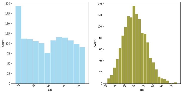
- 我们可以把年龄进行分组转换为年龄段
- BMI接近正态分布
# 箱线图
fig,axes=plt.subplots(1,2,figsize=(10,5))
sns.boxplot(x = 'age', data = health_ins_df, ax=axes[0])
sns.boxplot(x = 'bmi', data = health_ins_df, ax=axes[1])
plt.show()

可以看出BMI存在一些离群值 , 现在我们来看一下这些点
outlier_list = boxplot_stats(health_ins_df.bmi).pop(0)['fliers'].tolist()
print(outlier_list)
#查找包含异常值的行数
outlier_bmi_rows = health_ins_df[health_ins_df.bmi.isin(outlier_list)].shape[0]
print("bmi 中包含异常值的行数:", outlier_bmi_rows)

#离群值占比
#Percentage of rows which are outliers
percent_bmi_outlier = (outlier_bmi_rows/health_ins_df.shape[0])\*100
print("bmi离群值异常值的百分比 : ", percent_bmi_outlier)
[49.06, 48.07, 47.52, 47.41, 50.38, 47.6, 52.58, 47.74, 53.13]
bmi 中包含异常值的行数: 9
bmi离群值异常值的百分比 :  0.672645739910314
数值变量的数据转换
# 将年龄转换为分桶的
print("Minimum value for age : ", health_ins_df['age'].min(),"\nMaximum value for age : ", health_ins_df['age'].max())

'''
18至40岁的年龄将属于青年
41至58岁的年龄将低于中年
58岁以上将落入老年
'''
health_ins_df.loc[(health_ins_df['age'] >=18) & (health_ins_df['age'] <= 40), 'age\_group'] = '青年'
health_ins_df.loc[(health_ins_df['age'] >= 41) & (health_ins_df['age'] <= 58), 'age\_group'] = '中年'
health_ins_df.loc[health_ins_df['age'] > 58, 'age\_group'] = '老年'
Minimum value for age :  18
Maximum value for age :  64
# 去除BMI中的异常值
health_ins_df_clean = health_ins_df[~health_ins_df.bmi.isin(outlier_list)]
sns.boxplot(x = 'bmi', data = health_ins_df_clean)

对于分类型变量的分析
fig,axes=plt.subplots(1,5,figsize=(20,8))
sns.countplot(x = 'sex', data = health_ins_df_clean, palette = 'magma',ax=axes[0])
sns.countplot(x = 'children', data = health_ins_df_clean, palette = 'magma',ax=axes[1])
sns.countplot(x = 'smoker', data = health_ins_df_clean, palette = 'magma',ax=axes[2])
sns.countplot(x = 'region', data = health_ins_df_clean, palette = 'magma',ax=axes[3])
sns.countplot(x = 'age\_group', data = health_ins_df_clean, palette = 'magma',ax=axes[4])

数据准备完成后,下一阶段是建模。选择合适的算法将取决于数据的类型。例如,如果数据是连续的,您将应用回归建模,如果数据是分类的,您将应用分类算法建模。作为一名数据科学家,您将尝试许多模型来获得最合适的模型。
模型构建
在根据业务/技术限制选择正确的模型之前,尝试并测试数据集上所有可能的模型。在这个阶段,你也可以尝试一些 bagging 或 boosting 技术。在这里,我分别构建了线性回归模型、决策树回归、Gradient Boosting Regression.
简单的线性回归模型
在这里,我们首先使用线性回归模型作为基准模型。
from sklearn.linear_model import LinearRegression
lm = LinearRegression()
X = health_ins_df_processed.loc[:, health_ins_df_processed.columns != 'charges']#自闭哪里
y = health_ins_df_processed['charges']#因变量
X_train, X_test, y_train, y_test = train_test_split(X, y, test_size=0.33)#划分训练集和测试集


lm.fit(X_train,y_train)
print("R-Squared on train dataset={}".format(lm.score(X_train,y_train)))#训练集R2
lm.fit(X_test,y_test)
print("R-Squaredon test dataset={}".format(lm.score(X_test,y_test)))#测试集R2
R-Squared on train dataset=0.7494776882061486
R-Squaredon test dataset=0.7372938495110573
从结果来看,使用简单的线性回归
R
2
R^2
R2为0.74,说明模型解释了数据74%的信息,我们下面来看一些更complex的模型
决策树回归
X = health_ins_df_processed.loc[:, health_ins_df_processed.columns != 'charges']
y = health_ins_df_processed['charges']
X_train, X_test, y_train, y_test = train_test_split(X, y, test_size=0.33)
dtr = DecisionTreeRegressor(max_depth=4,min_samples_split=5,max_leaf_nodes=10)#初始化参数
dtr.fit(X_train,y_train)
print("R-Squared on train dataset={}".format(dtr.score(X_train,y_train)))#训练集R2

dtr.fit(X_test,y_test)
print("R-Squaredon test dataset={}".format(dtr.score(X_test,y_test)))#测试集R2
R-Squared on train dataset=0.8594291626976573
R-Squaredon test dataset=0.8571718114547656
上面的参数是我随机设定,大家还可以对其进行调参能提高一定的效果,调参的代码我上传到github上了https://github.com/JoJoYao996/data-science-projects
Gradient Boosting Regression
梯度提升回归模型的主要调整参数
- learning_rate:学习率,默认为0.1
- n_estimators:默认为100
- max_depth:单个回归估计器的最大深度。最大深度限制了树中的节点数。调整此参数以获得最佳性能;最佳值取决于输入变量的相互作用。值必须在 [1, inf) 范围内。
- min_samples_split:拆分内部节点所需的最小样本数:
- min_samples_leaf:叶节点最小样本数,这个参数会影响模型的平滑效果,尤其是在回归中。
我使用了gridsearch来分别对这些参数调整,下面是调参之后的结果。
#最终的模型
f_model = ensemble.GradientBoostingRegressor(learning_rate=0.015,n_estimators=250,max_depth=2,min_samples_leaf=5,
min_samples_split=2,subsample=1,loss = 'squared\_error')
f_model.fit(X_train, y_train)


**既有适合小白学习的零基础资料,也有适合3年以上经验的小伙伴深入学习提升的进阶课程,涵盖了95%以上大数据知识点,真正体系化!**
**由于文件比较多,这里只是将部分目录截图出来,全套包含大厂面经、学习笔记、源码讲义、实战项目、大纲路线、讲解视频,并且后续会持续更新**
**[需要这份系统化资料的朋友,可以戳这里获取](https://bbs.csdn.net/topics/618545628)**
(img-5dnFuRFd-1715715537688)]
[外链图片转存中...(img-QlW211WD-1715715537688)]
[外链图片转存中...(img-8wL0l3Yo-1715715537688)]
**既有适合小白学习的零基础资料,也有适合3年以上经验的小伙伴深入学习提升的进阶课程,涵盖了95%以上大数据知识点,真正体系化!**
**由于文件比较多,这里只是将部分目录截图出来,全套包含大厂面经、学习笔记、源码讲义、实战项目、大纲路线、讲解视频,并且后续会持续更新**
**[需要这份系统化资料的朋友,可以戳这里获取](https://bbs.csdn.net/topics/618545628)**


 被折叠的 条评论
为什么被折叠?
被折叠的 条评论
为什么被折叠?
 到【灌水乐园】发言


