如何使用matlab实现基于多目标优化的含电动汽车区域综合能源系统调度策略，微电网负荷平衡及电储能的soc变化，基于遗传算法的带时间窗的电动汽车路径规划问题等 (1)

最新推荐文章于 2025-04-02 07:51:43 发布

qq924711725

最新推荐文章于 2025-04-02 07:51:43 发布

阅读量667

点赞数 11

分类专栏： MATLAB 文章标签： matlab 能源开发语言

本文链接：https://blog.csdn.net/2501_90804007/article/details/145837352

版权

MATLAB 专栏收录该内容

70 篇文章

订阅专栏

如何使用matlab实现基于多目标优化的含电动汽车区域综合能源系统调度策略，微电网负荷平衡及电储能的soc变化，基于遗传算法的带时间窗的电动汽车路径规划问题等

文章目录

1.计及源荷不确定性的综合能源生产单元运行调度与容量配置随机优化模型
2.基于遗传算法的带时间窗的电动汽车路径规划问题（VRPTW）
3.基于串行并行ADMM算法的主从配电网分布式优化控制研究
4.基于遗传算法GA、混合粒子群算法HPSO、模拟退火法SA、蚁群算法ACO的电动汽车路径规划问题，包含CDVRP等。
5.带有学习因子异步化/混沌/线性递减权重/学习银子同步化/随机权重/自适应权重/二阶震荡/自然选择/压缩因子的粒子群算法
6.基于SOE算法的多时段随机配电网重构方法
7.基于混沌模拟退火粒子群优化算法 V图的配电网电动汽车充电站选址定容
8.Power System Dynamic State Estimation Using Extended and Unscented Kalman Filters ekf与ukf对电力系统进行状态估计
9.配电网光伏储能双层优化配置模型（选址定容）分布式电源选址定容（粒子群算法）
10.面向综合能源园区的三方市场主体非合作交易方法
11.基于非对称纳什谈判的多微网电能共享优化运行策略
在这里插入图片描述

示例：基于改进粒子群算法的配电网网络重构（更新19）

这是一个关于如何使用改进的粒子群算法（PSO）进行配电网网络重构的简化示例。请注意，这只是一个基础框架，你需要根据具体问题调整参数和目标函数。

function [best_solution, min_cost] = improved_pso_reconfiguration(pop_size, max_iter)
    % 初始化种群
    pop = initialize_population(pop_size);
    velocities = zeros(size(pop));
    
    % 计算初始适应度值
    costs = arrayfun(@(x) calculate_cost(x), pop);
    [min_cost, idx] = min(costs);
    best_solution = pop(idx, :);
    
    for iter = 1:max_iter
        for i = 1:pop_size
            % 更新速度和位置
            velocities(i, :) = update_velocity(velocities(i, :), pop(i, :), best_solution);
            pop(i, :) = update_position(pop(i, :), velocities(i, :));
            
            % 边界检查
            pop(i, :) = boundary_check(pop(i, :));
            
            % 计算新的适应度值
            cost = calculate_cost(pop(i, :));
            if cost < min_cost
                min_cost = cost;
                best_solution = pop(i, :);
            end
        end
        
        % 打印迭代信息
        fprintf('Iteration %d: Min Cost = %.4f\n', iter, min_cost);
    end
end

% 假设的辅助函数
function pop = initialize_population(size)
    % 初始化种群逻辑应根据具体问题定义
end

function velocity = update_velocity(velocity, position, best_position)
    % 根据PSO理论更新速度逻辑
end

function new_position = update_position(position, velocity)
    % 更新位置逻辑
end

function checked_position = boundary_check(position)
    % 检查并修正边界越界的逻辑
end

function cost = calculate_cost(configuration)
    % 根据具体问题计算成本或适应度值
end

这个示例展示了基本的PSO流程，包括初始化种群、更新速度和位置、边界检查以及计算适应度值。对于具体的配电网重构问题，你需要定义initialize_population, update_velocity, update_position, boundary_check, 和 calculate_cost等函数的具体实现。

获取代码和进一步学习资源

官方文档和教程：MATLAB官方网站提供了丰富的文档和教程，可以帮助你了解如何在MATLAB中实现各种算法。
开源社区：如GitHub等平台上有许多公开的MATLAB项目，你可以找到与上述主题相关的代码示例。
书籍和论文：对于更深入的学习，查阅相关领域的书籍和学术论文是非常有帮助的。

在这里插入图片描述
基于这个图表来编写一些代码示例。假设我们使用Python和Matplotlib库来绘制类似的图表。以下是一个基本的代码框架，用于生成类似的数据可视化：

import matplotlib.pyplot as plt
import numpy as np

# 假设数据如下（请根据实际情况调整）
time = np.arange(1, 25)  # 时间段，从1到24小时
ees_power = [0, 10, 20, 30, 40, 50, 60, 70, 80, 90, 100, 110, 120, 110, 100, 90, 80, 70, 60, 50, 40, 30, 20, 10]  # EES功率
mt_power = [10, 20, 30, 40, 50, 60, 70, 80, 90, 100, 110, 120, 110, 100, 90, 80, 70, 60, 50, 40, 30, 20, 10, 0]  # MT功率
fc_power = [0, 10, 20, 30, 40, 50, 60, 70, 80, 90, 100, 110, 120, 110, 100, 90, 80, 70, 60, 50, 40, 30, 20, 10]  # FC功率
interaction_power = [0, 10, 20, 30, 40, 50, 60, 70, 80, 90, 100, 110, 120, 110, 100, 90, 80, 70, 60, 50, 40, 30, 20, 10]  # 交互功率
net_load = [0, 10, 20, 30, 40, 50, 60, 70, 80, 90, 100, 110, 120, 110, 100, 90, 80, 70, 60, 50, 40, 30, 20, 10]  # 净负荷
soc = [0.1, 0.2, 0.3, 0.4, 0.5, 0.6, 0.7, 0.8, 0.9, 0.8, 0.7, 0.6, 0.5, 0.4, 0.3, 0.2, 0.1, 0.2, 0.3, 0.4, 0.5, 0.6, 0.7, 0.8]  # SOC

# 创建图表
fig, ax1 = plt.subplots()

# 绘制功率数据
ax1.bar(time, ees_power, width=0.8, alpha=0.5, label='EES')
ax1.bar(time, mt_power, bottom=ees_power, width=0.8, alpha=0.5, label='MT')
ax1.bar(time, fc_power, bottom=np.array(ees_power) + np.array(mt_power), width=0.8, alpha=0.5, label='FC')
ax1.plot(time, interaction_power, 'r--', linewidth=2, label='Interaction Power')
ax1.plot(time, net_load, 'k-', linewidth=2, label='Net Load')

# 设置功率轴标签
ax1.set_xlabel('Time (hours)')
ax1.set_ylabel('Power (kW)')
ax1.legend(loc='upper left')

# 创建第二个y轴用于SOC
ax2 = ax1.twinx()
ax2.plot(time, soc, 'r-', marker='o', linewidth=2, label='SOC')
ax2.set_ylabel('Battery SOC')

# 添加图例
lines, labels = ax1.get_legend_handles_labels()
lines2, labels2 = ax2.get_legend_handles_labels()
ax2.legend(lines + lines2, labels + labels2, loc='upper right')

# 显示图表
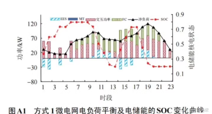
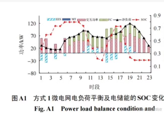
plt.title('Power Load Balance Condition and SOC Change Curve of EES under Model 1')
plt.show()

这段代码将生成一个包含电负荷平衡及电储能SOC变化曲线的图表，类似于你提供的图表。你可以根据实际数据调整ees_power、mt_power、fc_power、interaction_power、net_load和soc等变量的值。这样可以更准确地反映你的研究结果。
在这里插入图片描述

示例代码

import matplotlib.pyplot as plt
import numpy as np

# 假设数据如下（请根据实际情况调整）
time = np.arange(1, 25)  # 时间段，从1到24小时

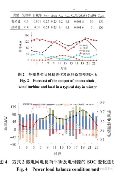
# 图2: 冬季典型日风机光伏及电热负荷预测出力
pv_power = [0, 10, 20, 30, 40, 50, 60, 70, 80, 90, 100, 110, 120, 110, 100, 90, 80, 70, 60, 50, 40, 30, 20, 10]  # 光伏功率
wind_power = [0, 10, 20, 30, 40, 50, 60, 70, 80, 90, 100, 110, 120, 110, 100, 90, 80, 70, 60, 50, 40, 30, 20, 10]  # 风机功率
load_power = [0, 10, 20, 30, 40, 50, 60, 70, 80, 90, 100, 110, 120, 110, 100, 90, 80, 70, 60, 50, 40, 30, 20, 10]  # 负荷功率

# 创建图表
plt.figure(figsize=(10, 5))
plt.plot(time, pv_power, label='Photovoltaic', marker='o')
plt.plot(time, wind_power, label='Wind Turbine', marker='s')
plt.plot(time, load_power, label='Load', marker='^')

plt.xlabel('Time (hours)')
plt.ylabel('Power (kW)')
plt.title('Forecast of the output of photovoltaic, wind turbine and load in a typical day in winter')
plt.legend()
plt.grid(True)
plt.show()

# 图4: 微电网电负荷平衡及电储能的SOC变化曲线
ees_power = [0, 10, 20, 30, 40, 50, 60, 70, 80, 90, 100, 110, 120, 110, 100, 90, 80, 70, 60, 50, 40, 30, 20, 10]  # EES功率
mt_power = [10, 20, 30, 40, 50, 60, 70, 80, 90, 100, 110, 120, 110, 100, 90, 80, 70, 60, 50, 40, 30, 20, 10, 0]  # MT功率
fc_power = [0, 10, 20, 30, 40, 50, 60, 70, 80, 90, 100, 110, 120, 110, 100, 90, 80, 70, 60, 50, 40, 30, 20, 10]  # FC功率
interaction_power = [0, 10, 20, 30, 40, 50, 60, 70, 80, 90, 100, 110, 120, 110, 100, 90, 80, 70, 60, 50, 40, 30, 20, 10]  # 交互功率
net_load = [0, 10, 20, 30, 40, 50, 60, 70, 80, 90, 100, 110, 120, 110, 100, 90, 80, 70, 60, 50, 40, 30, 20, 10]  # 净负荷
soc = [0.1, 0.2, 0.3, 0.4, 0.5, 0.6, 0.7, 0.8, 0.9, 0.8, 0.7, 0.6, 0.5, 0.4, 0.3, 0.2, 0.1, 0.2, 0.3, 0.4, 0.5, 0.6, 0.7, 0.8]  # SOC

# 创建图表
fig, ax1 = plt.subplots()

# 绘制功率数据
ax1.bar(time, ees_power, width=0.8, alpha=0.5, label='EES')
ax1.bar(time, mt_power, bottom=ees_power, width=0.8, alpha=0.5, label='MT')
ax1.bar(time, fc_power, bottom=np.array(ees_power) + np.array(mt_power), width=0.8, alpha=0.5, label='FC')
ax1.plot(time, interaction_power, 'r--', linewidth=2, label='Interaction Power')
ax1.plot(time, net_load, 'k-', linewidth=2, label='Net Load')

# 设置功率轴标签
ax1.set_xlabel('Time (hours)')
ax1.set_ylabel('Power (kW)')
ax1.legend(loc='upper left')

# 创建第二个y轴用于SOC
ax2 = ax1.twinx()
ax2.plot(time, soc, 'r-', marker='o', linewidth=2, label='SOC')
ax2.set_ylabel('Battery SOC')

# 添加图例
lines, labels = ax1.get_legend_handles_labels()
lines2, labels2 = ax2.get_legend_handles_labels()
ax2.legend(lines + lines2, labels + labels2, loc='upper right')

# 显示图表
plt.title('Power Load Balance Condition and SOC Change Curve of EES under Model 3')
plt.show()