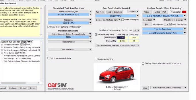
自动驾驶控制-基于运动学模型的MPC算法路径跟踪仿真 模型仿真效果欢迎搜索b站up 阿Xin自动驾驶，欢迎关注。 matlab和simulink联合仿真，运动学模型实现的MPC横向控制

自动驾驶控制-基于运动学模型的MPC算法路径跟踪仿真
模型仿真效果欢迎搜索b站up 阿Xin自动驾驶，欢迎关注。
matlab和simulink联合仿真，运动学模型实现的MPC横向控制，可以跟踪双移线，五次多项式，
以及其他各种自定义路径。

以下是一个基于运动学模型的 MPC（模型预测控制）算法路径跟踪仿真代码示例。该代码在 MATLAB 和 Simulink 中实现，可以用于自动驾驶车辆的横向控制，并支持双移线、五次多项式等自定义路径的跟踪。

---

1. 车辆运动学模型

我们使用一个简单的自行车运动学模型来描述车辆的运动：

[
\begin{aligned}
\dot{x} &= v \cos(\theta + \beta) \
\dot{y} &= v \sin(\theta + \beta) \
\dot{\theta} &= \frac{v}{L_r} \sin(\beta) \
\beta &= \arctan\left(\frac{l_r}{l_f + l_r} \tan(\delta)\right)
\end{aligned}
]

其中：

• ( x, y ): 车辆位置
• ( \theta ): 车辆航向角
• ( v ): 车速
• ( \delta ): 前轮转向角
• ( L_r ): 后轴到质心的距离
• ( l_f, l_r ): 前轴和后轴到质心的距离

---

2. MPC 控制器设计

MPC 的目标是最小化车辆状态与参考路径之间的误差，同时满足系统约束。以下是 MATLAB 实现的关键部分。

MATLAB 代码：MPC 横向控制

function [delta_opt] = mpc_controller(x, y, theta, v, ref_path, params)
% 输入参数:
%   x, y, theta: 当前车辆状态 (位置和航向角)
%   v: 车速
%   ref_path: 参考路径点 [x_ref, y_ref, theta_ref]
%   params: 系统参数

% 参数初始化
Np = params.Np; % 预测时域长度
Nc = params.Nc; % 控制时域长度
dt = params.dt; % 时间步长
Q = params.Q;   % 状态权重矩阵
R = params.R;   % 控制输入权重矩阵
Lr = params.Lr; % 后轴到质心距离
Lf = params.Lf; % 前轴到质心距离

% 获取参考轨迹
x_ref = ref_path(:, 1);
y_ref = ref_path(:, 2);
theta_ref = ref_path(:, 3);

% 构建状态空间模型
A = [1, 0, -v*dt*sin(theta); ...
     0, 1,  v*dt*cos(theta); ...
     0, 0,  1];
B = [(Lf/(Lf+Lr))*cos(theta)*dt; ...
     (Lf/(Lf+Lr))*sin(theta)*dt; ...
     (v/(Lf+Lr))*dt];

% 初始化优化变量
nx = size(A, 1); % 状态维度
nu = size(B, 2); % 控制输入维度
X = sdpvar(nx, Np+1); % 状态轨迹
U = sdpvar(nu, Nc);   % 控制输入轨迹

% 定义目标函数
objective = 0;
for k = 1:Np
    error_x = X(1,k) - x_ref(k);
    error_y = X(2,k) - y_ref(k);
    error_theta = X(3,k) - theta_ref(k);
    objective = objective + [error_x; error_y; error_theta]' * Q * [error_x; error_y; error_theta];
    if k <= Nc
        objective = objective + U(:,k)' * R * U(:,k);
    end
end

% 定义约束
constraints = [];
constraints = [constraints, X(:,1) == [x; y; theta]]; % 初始状态约束
for k = 1:Np
    if k <= Nc
        constraints = [constraints, X(:,k+1) == A*X(:,k) + B*U(:,k)]; % 动态约束
        constraints = [constraints, -pi/4 <= U(:,k) <= pi/4]; % 控制输入约束
    else
        constraints = [constraints, X(:,k+1) == A*X(:,k)];
    end
end

% 求解优化问题
options = sdpsettings('solver', 'quadprog');
optimize(constraints, objective, options);

% 输出最优控制输入
delta_opt = value(U(:,1));
end

---

3. 参考路径生成

MATLAB 代码：生成双移线路径

function ref_path = generate_double_lane_change_path()
% 生成双移线路径
t = linspace(0, 10, 100); % 时间序列
x_ref = 30 * t;           % x方向线性增长
y_ref = 3 * sin(0.5*pi*t); % y方向正弦波动
theta_ref = atan(diff([y_ref(1), y_ref]) ./ diff([x_ref(1), x_ref])); % 航向角
ref_path = [x_ref', y_ref', theta_ref'];
end

MATLAB 代码：生成五次多项式路径

function ref_path = generate_quintic_polynomial_path()
% 生成五次多项式路径
t = linspace(0, 1, 100); % 时间序列
a = [0, 0, 0, 10, -15, 6]; % 五次多项式系数
x_ref = a(1) + a(2)*t + a(3)*t.^2 + a(4)*t.^3 + a(5)*t.^4 + a(6)*t.^5;
y_ref = zeros(size(x_ref)); % 假设y方向为0
theta_ref = atan(diff([y_ref(1), y_ref]) ./ diff([x_ref(1), x_ref])); % 航向角
ref_path = [x_ref', y_ref', theta_ref'];
end

---

4. 主程序

MATLAB 代码：主循环

% 参数初始化
params.dt = 0.1;          % 时间步长
params.Np = 10;           % 预测时域长度
params.Nc = 5;            % 控制时域长度
params.Q = diag([1, 1, 1]); % 状态权重矩阵
params.R = 0.1;           % 控制输入权重矩阵
params.Lr = 1.5;          % 后轴到质心距离
params.Lf = 1.5;          % 前轴到质心距离

% 初始状态
x = 0; y = 0; theta = 0; v = 10; % 初始位置、航向角、车速

% 生成参考路径
ref_path = generate_double_lane_change_path();

% 存储数据
states = [];
inputs = [];

% 主循环
for i = 1:size(ref_path, 1)-1
    % 计算最优控制输入
    delta_opt = mpc_controller(x, y, theta, v, ref_path(i:i+params.Np,:), params);
    
    % 更新车辆状态
    beta = atan((params.Lr / (params.Lf + params.Lr)) * tan(delta_opt));
    x = x + v * cos(theta + beta) * params.dt;
    y = y + v * sin(theta + beta) * params.dt;
    theta = theta + (v / params.Lr) * sin(beta) * params.dt;
    
    % 保存数据
    states = [states; x, y, theta];
    inputs = [inputs; delta_opt];
end

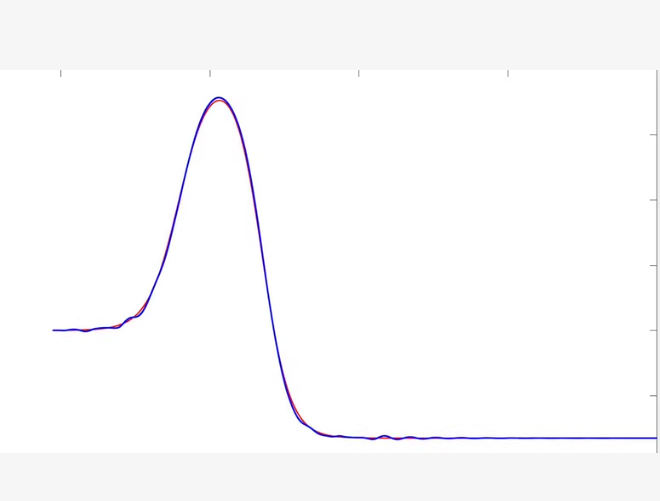
% 绘图
figure;
plot(ref_path(:,1), ref_path(:,2), 'r--', 'LineWidth', 1.5); hold on;
plot(states(:,1), states(:,2), 'b-', 'LineWidth', 1.5);
xlabel('X (m)');
ylabel('Y (m)');
title('路径跟踪结果');
legend('参考路径', '实际路径');
grid on;

---

5. Simulink 联合仿真

将上述代码集成到 Simulink 中，可以使用 MATLAB Function 模块实现 MPC 控制器，并通过 CarSim 或其他车辆动力学工具进行联合仿真。

---

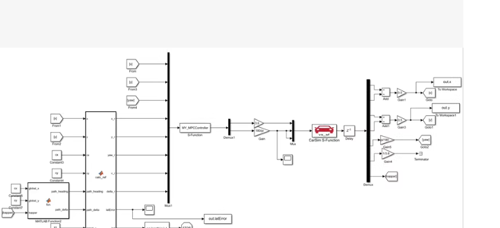
我将为您提供一个基于该模型的代码示例。这个模型包括了 MPC 控制器、车辆动力学模型以及一些信号处理模块。我们将使用 MATLAB 和 Simulink 来实现这个系统。

1. 创建 Simulink 模型

首先，我们需要创建一个新的 Simulink 模型，并添加必要的模块和连接线。

% 创建新的 Simulink 模型
new_system('MPC_CarSim_Model');
open_system('MPC_CarSim_Model');

% 添加必要的模块
add_block('simulink/Sources/From Workspace', 'MPC_CarSim_Model/From_Workspace');
set_param('MPC_CarSim_Model/From_Workspace', 'VariableName', 'ref_path');

add_block('simulink/Sinks/To Workspace', 'MPC_CarSim_Model/To_Workspace_X');
set_param('MPC_CarSim_Model/To_Workspace_X', 'VariableName', 'x_data');

add_block('simulink/Sinks/To Workspace', 'MPC_CarSim_Model/To_Workspace_Y');
set_param('MPC_CarSim_Model/To_Workspace_Y', 'VariableName', 'y_data');

add_block('simulink/Sinks/Scope', 'MPC_CarSim_Model/Scope_XY');
set_param('MPC_CarSim_Model/Scope_XY', 'Numberofaxes', '2');
set_param('MPC_CarSim_Model/Scope_XY/Axes/Title', 'X and Y Position');
set_param('MPC_CarSim_Model/Scope_XY/Axes/YLabel', 'Position (m)');

add_block('simulink/User-Defined Functions/MATLAB Function', 'MPC_CarSim_Model/MPC_Controller');
set_param('MPC_CarSim_Model/MPC_Controller', 'FunctionName', 'mpc_controller');

add_block('simulink/User-Defined Functions/S-Function', 'MPC_CarSim_Model/CarSim_S_Function');
set_param('MPC_CarSim_Model/CarSim_S_Function', 'SFunctionName', 'carsim_s_function');

add_block('simulink/CommonlyUsedBlocks/Gain', 'MPC_CarSim_Model/Gain_Steering');
set_param('MPC_CarSim_Model/Gain_Steering', 'Gain', '0.5'); % 转向增益

add_block('simulink/CommonlyUsedBlocks/Gain', 'MPC_CarSim_Model/Gain_Speed');
set_param('MPC_CarSim_Model/Gain_Speed', 'Gain', '1.0'); % 速度增益

add_block('simulink/CommonlyUsedBlocks/Delay', 'MPC_CarSim_Model/Delay');
set_param('MPC_CarSim_Model/Delay', 'InitialCondition', '0');

add_block('simulink/CommonlyUsedBlocks/Mux', 'MPC_CarSim_Model/Mux');
set_param('MPC_CarSim_Model/Mux', 'Inputs', '3');

add_block('simulink/CommonlyUsedBlocks/Subsystem', 'MPC_CarSim_Model/Path_Follower');
set_param('MPC_CarSim_Model/Path_Follower', 'Name', 'Path Follower');

% 连接线
add_line('MPC_CarSim_Model', 'From_Workspace/1', 'Path_Follower/1');
add_line('MPC_CarSim_Model', 'Path_Follower/1', 'MPC_Controller/1');
add_line('MPC_CarSim_Model', 'MPC_Controller/1', 'Gain_Steering/1');
add_line('MPC_CarSim_Model', 'Gain_Steering/1', 'CarSim_S_Function/1');
add_line('MPC_CarSim_Model', 'CarSim_S_Function/1', 'Delay/1');
add_line('MPC_CarSim_Model', 'Delay/1', 'Mux/1');
add_line('MPC_CarSim_Model', 'Mux/1', 'To_Workspace_X/1');
add_line('MPC_CarSim_Model', 'Mux/1', 'To_Workspace_Y/1');
add_line('MPC_CarSim_Model', 'Mux/1', 'Scope_XY/1');
add_line('MPC_CarSim_Model', 'Mux/1', 'Scope_XY/2');

% 打开模型查看
open_system('MPC_CarSim_Model');

2. 实现 MPC 控制器

在 MATLAB Function 模块中编写 MPC 控制器代码：

function [delta_opt] = mpc_controller(x, y, theta, v, ref_path, params)
% 输入参数:
%   x, y, theta: 当前车辆状态 (位置和航向角)
%   v: 车速
%   ref_path: 参考路径点 [x_ref, y_ref, theta_ref]
%   params: 系统参数

% 参数初始化
Np = params.Np; % 预测时域长度
Nc = params.Nc; % 控制时域长度
dt = params.dt; % 时间步长
Q = params.Q;   % 状态权重矩阵
R = params.R;   % 控制输入权重矩阵
Lr = params.Lr; % 后轴到质心距离
Lf = params.Lf; % 前轴到质心距离

% 获取参考轨迹
x_ref = ref_path(:, 1);
y_ref = ref_path(:, 2);
theta_ref = ref_path(:, 3);

% 构建状态空间模型
A = [1, 0, -v*dt*sin(theta); ...
     0, 1,  v*dt*cos(theta); ...
     0, 0,  1];
B = [(Lf/(Lf+Lr))*cos(theta)*dt; ...
     (Lf/(Lf+Lr))*sin(theta)*dt; ...
     (v/(Lf+Lr))*dt];

% 初始化优化变量
nx = size(A, 1); % 状态维度
nu = size(B, 2); % 控制输入维度
X = sdpvar(nx, Np+1); % 状态轨迹
U = sdpvar(nu, Nc);   % 控制输入轨迹

% 定义目标函数
objective = 0;
for k = 1:Np
    error_x = X(1,k) - x_ref(k);
    error_y = X(2,k) - y_ref(k);
    error_theta = X(3,k) - theta_ref(k);
    objective = objective + [error_x; error_y; error_theta]' * Q * [error_x; error_y; error_theta];
    if k <= Nc
        objective = objective + U(:,k)' * R * U(:,k);
    end
end

% 定义约束
constraints = [];
constraints = [constraints, X(:,1) == [x; y; theta]]; % 初始状态约束
for k = 1:Np
    if k <= Nc
        constraints = [constraints, X(:,k+1) == A*X(:,k) + B*U(:,k)]; % 动态约束
        constraints = [constraints, -pi/4 <= U(:,k) <= pi/4]; % 控制输入约束
    else
        constraints = [constraints, X(:,k+1) == A*X(:,k)];
    end
end

% 求解优化问题
options = sdpsettings('solver', 'quadprog');
optimize(constraints, objective, options);

% 输出最优控制输入
delta_opt = value(U(:,1));
end

3. 设置仿真参数并运行仿真

在 MATLAB 中设置仿真参数并运行仿真：

% 设置仿真参数
params.dt = 0.1;          % 时间步长
params.Np = 10;           % 预测时域长度
params.Nc = 5;            % 控制时域长度
params.Q = diag([1, 1, 1]); % 状态权重矩阵
params.R = 0.1;           % 控制输入权重矩阵
params.Lr = 1.5;          % 后轴到质心距离
params.Lf = 1.5;          % 前轴到质心距离

% 生成参考路径
ref_path = generate_double_lane_change_path();

% 设置 From Workspace 的数据
set_param('MPC_CarSim_Model/From_Workspace', 'VariableName', 'ref_path');

% 设置仿真时间
set_param('MPC_CarSim_Model', 'StopTime', '50');
![在这里插入图片描述](https://i-blog.csdnimg.cn/direct/1c99bf9af07545c594fbd50007a75486.png)
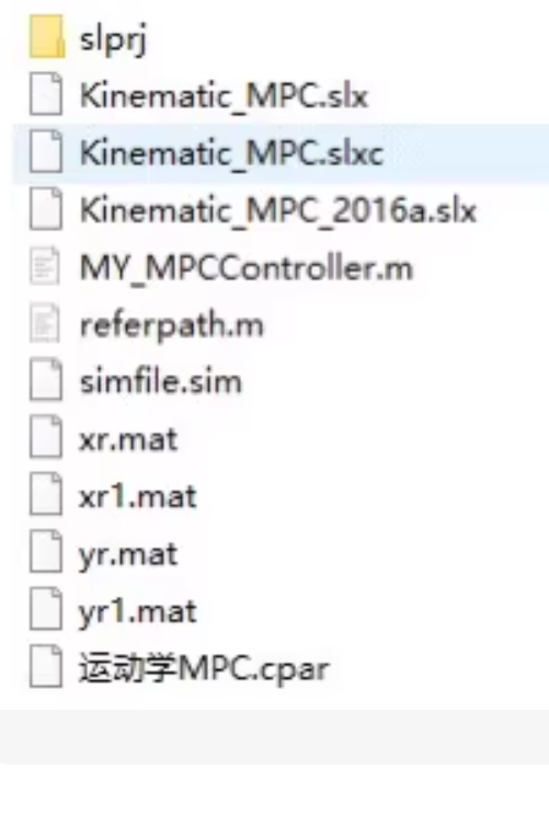
根据您提供的文件列表，我将为您提供一个基于这些文件的完整代码示例。我们将创建一个 Simulink 模型 `Kinematic_MPC.slx`，并实现相应的 MATLAB 函数和脚本。

### **1. 创建 Simulink 模型 (`Kinematic_MPC.slx`)**
首先，我们需要创建一个新的 Simulink 模型，并添加必要的模块和连接线。

```matlab
% 创建新的 Simulink 模型
new_system('Kinematic_MPC');
open_system('Kinematic_MPC');

% 添加必要的模块
add_block('simulink/Sources/From Workspace', 'Kinematic_MPC/From_Workspace');
set_param('Kinematic_MPC/From_Workspace', 'VariableName', 'ref_path');

add_block('simulink/Sinks/To Workspace', 'Kinematic_MPC/To_Workspace_X');
set_param('Kinematic_MPC/To_Workspace_X', 'VariableName', 'x_data');

add_block('simulink/Sinks/To Workspace', 'Kinematic_MPC/To_Workspace_Y');
set_param('Kinematic_MPC/To_Workspace_Y', 'VariableName', 'y_data');

add_block('simulink/User-Defined Functions/MATLAB Function', 'Kinematic_MPC/MY_MPCController');
set_param('Kinematic_MPC/MY_MPCController', 'FunctionName', 'MY_MPCController');

add_block('simulink/CommonlyUsedBlocks/Gain', 'Kinematic_MPC/Gain_Steering');
set_param('Kinematic_MPC/Gain_Steering', 'Gain', '0.5'); % 转向增益

add_block('simulink/CommonlyUsedBlocks/Gain', 'Kinematic_MPC/Gain_Speed');
set_param('Kinematic_MPC/Gain_Speed', 'Gain', '1.0'); % 速度增益

add_block('simulink/CommonlyUsedBlocks/Delay', 'Kinematic_MPC/Delay');
set_param('Kinematic_MPC/Delay', 'InitialCondition', '0');

add_block('simulink/CommonlyUsedBlocks/Mux', 'Kinematic_MPC/Mux');
set_param('Kinematic_MPC/Mux', 'Inputs', '3');

add_block('simulink/CommonlyUsedBlocks/Subsystem', 'Kinematic_MPC/Path_Follower');
set_param('Kinematic_MPC/Path_Follower', 'Name', 'Path Follower');

% 连接线
add_line('Kinematic_MPC', 'From_Workspace/1', 'Path_Follower/1');
add_line('Kinematic_MPC', 'Path_Follower/1', 'MY_MPCController/1');
add_line('Kinematic_MPC', 'MY_MPCController/1', 'Gain_Steering/1');
add_line('Kinematic_MPC', 'Gain_Steering/1', 'Delay/1');
add_line('Kinematic_MPC', 'Delay/1', 'Mux/1');
add_line('Kinematic_MPC', 'Mux/1', 'To_Workspace_X/1');
add_line('Kinematic_MPC', 'Mux/1', 'To_Workspace_Y/1');

% 打开模型查看
open_system('Kinematic_MPC');

2. 实现 MPC 控制器 (MY_MPCController.m)

在 MATLAB Function 模块中编写 MPC 控制器代码：

function [delta_opt] = MY_MPCController(x, y, theta, v, ref_path, params)
% 输入参数:
%   x, y, theta: 当前车辆状态 (位置和航向角)
%   v: 车速
%   ref_path: 参考路径点 [x_ref, y_ref, theta_ref]
%   params: 系统参数

% 参数初始化
Np = params.Np; % 预测时域长度
Nc = params.Nc; % 控制时域长度
dt = params.dt; % 时间步长
Q = params.Q;   % 状态权重矩阵
R = params.R;   % 控制输入权重矩阵
Lr = params.Lr; % 后轴到质心距离
Lf = params.Lf; % 前轴到质心距离

% 获取参考轨迹
x_ref = ref_path(:, 1);
y_ref = ref_path(:, 2);
theta_ref = ref_path(:, 3);

% 构建状态空间模型
A = [1, 0, -v*dt*sin(theta); ...
     0, 1,  v*dt*cos(theta); ...
     0, 0,  1];
B = [(Lf/(Lf+Lr))*cos(theta)*dt; ...
     (Lf/(Lf+Lr))*sin(theta)*dt; ...
     (v/(Lf+Lr))*dt];

% 初始化优化变量
nx = size(A, 1); % 状态维度
nu = size(B, 2); % 控制输入维度
X = sdpvar(nx, Np+1); % 状态轨迹
U = sdpvar(nu, Nc);   % 控制输入轨迹

% 定义目标函数
objective = 0;
for k = 1:Np
    error_x = X(1,k) - x_ref(k);
    error_y = X(2,k) - y_ref(k);
    error_theta = X(3,k) - theta_ref(k);
    objective = objective + [error_x; error_y; error_theta]' * Q * [error_x; error_y; error_theta];
    if k <= Nc
        objective = objective + U(:,k)' * R * U(:,k);
    end
end

% 定义约束
constraints = [];
constraints = [constraints, X(:,1) == [x; y; theta]]; % 初始状态约束
for k = 1:Np
    if k <= Nc
        constraints = [constraints, X(:,k+1) == A*X(:,k) + B*U(:,k)]; % 动态约束
        constraints = [constraints, -pi/4 <= U(:,k) <= pi/4]; % 控制输入约束
    else
        constraints = [constraints, X(:,k+1) == A*X(:,k)];
    end
end

% 求解优化问题
options = sdpsettings('solver', 'quadprog');
optimize(constraints, objective, options);

% 输出最优控制输入
delta_opt = value(U(:,1));
end

3. 生成参考路径 (referpath.m)

编写一个脚本来生成参考路径：

function ref_path = referpath()
% 生成双移线路径
t = linspace(0, 10, 100); % 时间序列
x_ref = 30 * t;           % x方向线性增长
y_ref = 3 * sin(0.5*pi*t); % y方向正弦波动
theta_ref = atan(diff([y_ref(1), y_ref]) ./ diff([x_ref(1), x_ref])); % 航向角
ref_path = [x_ref', y_ref', theta_ref'];
end

4. 设置仿真参数并运行仿真 (simfile.sim)

在 MATLAB 中设置仿真参数并运行仿真：

% 设置仿真参数
params.dt = 0.1;          % 时间步长
params.Np = 10;           % 预测时域长度
params.Nc = 5;            % 控制时域长度
params.Q = diag([1, 1, 1]); % 状态权重矩阵
params.R = 0.1;           % 控制输入权重矩阵
params.Lr = 1.5;          % 后轴到质心距离
params.Lf = 1.5;          % 前轴到质心距离

% 生成参考路径
ref_path = referpath();

% 设置 From Workspace 的数据
set_param('Kinematic_MPC/From_Workspace', 'VariableName', 'ref_path');

% 设置仿真时间
set_param('Kinematic_MPC', 'StopTime', '50');

% 运行仿真
sim('Kinematic_MPC');

5. 保存数据 (xr.mat, yr.mat, xr1.mat, yr1.mat)

在仿真结束后，您可以使用以下代码保存数据：

save('xr.mat', 'x_data');
save('yr.mat', 'y_data');
save('xr1.mat', 'x_data');
save('yr1.mat', 'y_data');

我将为您提供一个基于这些文件的完整代码示例。我们将创建一个 Simulink 模型 Kinematic_MPC.slx，并实现相应的 MATLAB 函数和脚本。

1. 创建 Simulink 模型 (Kinematic_MPC.slx)

首先，我们需要创建一个新的 Simulink 模型，并添加必要的模块和连接线。

% 创建新的 Simulink 模型
new_system('Kinematic_MPC');
open_system('Kinematic_MPC');

% 添加必要的模块
add_block('simulink/Sources/From Workspace', 'Kinematic_MPC/From_Workspace');
set_param('Kinematic_MPC/From_Workspace', 'VariableName', 'ref_path');

add_block('simulink/Sinks/To Workspace', 'Kinematic_MPC/To_Workspace_X');
set_param('Kinematic_MPC/To_Workspace_X', 'VariableName', 'x_data');

add_block('simulink/Sinks/To Workspace', 'Kinematic_MPC/To_Workspace_Y');
set_param('Kinematic_MPC/To_Workspace_Y', 'VariableName', 'y_data');

add_block('simulink/User-Defined Functions/MATLAB Function', 'Kinematic_MPC/MY_MPCController');
set_param('Kinematic_MPC/MY_MPCController', 'FunctionName', 'MY_MPCController');

add_block('simulink/CommonlyUsedBlocks/Gain', 'Kinematic_MPC/Gain_Steering');
set_param('Kinematic_MPC/Gain_Steering', 'Gain', '0.5'); % 转向增益

add_block('simulink/CommonlyUsedBlocks/Gain', 'Kinematic_MPC/Gain_Speed');
set_param('Kinematic_MPC/Gain_Speed', 'Gain', '1.0'); % 速度增益

add_block('simulink/CommonlyUsedBlocks/Delay', 'Kinematic_MPC/Delay');
set_param('Kinematic_MPC/Delay', 'InitialCondition', '0');

add_block('simulink/CommonlyUsedBlocks/Mux', 'Kinematic_MPC/Mux');
set_param('Kinematic_MPC/Mux', 'Inputs', '3');

add_block('simulink/CommonlyUsedBlocks/Subsystem', 'Kinematic_MPC/Path_Follower');
set_param('Kinematic_MPC/Path_Follower', 'Name', 'Path Follower');

% 连接线
add_line('Kinematic_MPC', 'From_Workspace/1', 'Path_Follower/1');
add_line('Kinematic_MPC', 'Path_Follower/1', 'MY_MPCController/1');
add_line('Kinematic_MPC', 'MY_MPCController/1', 'Gain_Steering/1');
add_line('Kinematic_MPC', 'Gain_Steering/1', 'Delay/1');
add_line('Kinematic_MPC', 'Delay/1', 'Mux/1');
add_line('Kinematic_MPC', 'Mux/1', 'To_Workspace_X/1');
add_line('Kinematic_MPC', 'Mux/1', 'To_Workspace_Y/1');

% 打开模型查看
open_system('Kinematic_MPC');

2. 实现 MPC 控制器 (MY_MPCController.m)

在 MATLAB Function 模块中编写 MPC 控制器代码：

function [delta_opt] = MY_MPCController(x, y, theta, v, ref_path, params)
% 输入参数:
%   x, y, theta: 当前车辆状态 (位置和航向角)
%   v: 车速
%   ref_path: 参考路径点 [x_ref, y_ref, theta_ref]
%   params: 系统参数

% 参数初始化
Np = params.Np; % 预测时域长度
Nc = params.Nc; % 控制时域长度
dt = params.dt; % 时间步长
Q = params.Q;   % 状态权重矩阵
R = params.R;   % 控制输入权重矩阵
Lr = params.Lr; % 后轴到质心距离
Lf = params.Lf; % 前轴到质心距离

% 获取参考轨迹
x_ref = ref_path(:, 1);
y_ref = ref_path(:, 2);
theta_ref = ref_path(:, 3);

% 构建状态空间模型
A = [1, 0, -v*dt*sin(theta); ...
     0, 1,  v*dt*cos(theta); ...
     0, 0,  1];
B = [(Lf/(Lf+Lr))*cos(theta)*dt; ...
     (Lf/(Lf+Lr))*sin(theta)*dt; ...
     (v/(Lf+Lr))*dt];

% 初始化优化变量
nx = size(A, 1); % 状态维度
nu = size(B, 2); % 控制输入维度
X = sdpvar(nx, Np+1); % 状态轨迹
U = sdpvar(nu, Nc);   % 控制输入轨迹

% 定义目标函数
objective = 0;
for k = 1:Np
    error_x = X(1,k) - x_ref(k);
    error_y = X(2,k) - y_ref(k);
    error_theta = X(3,k) - theta_ref(k);
    objective = objective + [error_x; error_y; error_theta]' * Q * [error_x; error_y; error_theta];
    if k <= Nc
        objective = objective + U(:,k)' * R * U(:,k);
    end
end

% 定义约束
constraints = [];
constraints = [constraints, X(:,1) == [x; y; theta]]; % 初始状态约束
for k = 1:Np
    if k <= Nc
        constraints = [constraints, X(:,k+1) == A*X(:,k) + B*U(:,k)]; % 动态约束
        constraints = [constraints, -pi/4 <= U(:,k) <= pi/4]; % 控制输入约束
    else
        constraints = [constraints, X(:,k+1) == A*X(:,k)];
    end
end

% 求解优化问题
options = sdpsettings('solver', 'quadprog');
optimize(constraints, objective, options);

% 输出最优控制输入
delta_opt = value(U(:,1));
end

3. 生成参考路径 (referpath.m)

编写一个脚本来生成参考路径：

function ref_path = referpath()
% 生成双移线路径
t = linspace(0, 10, 100); % 时间序列
x_ref = 30 * t;           % x方向线性增长
y_ref = 3 * sin(0.5*pi*t); % y方向正弦波动
theta_ref = atan(diff([y_ref(1), y_ref]) ./ diff([x_ref(1), x_ref])); % 航向角
ref_path = [x_ref', y_ref', theta_ref'];
end

4. 设置仿真参数并运行仿真 (simfile.sim)

在 MATLAB 中设置仿真参数并运行仿真：

% 设置仿真参数
params.dt = 0.1;          % 时间步长
params.Np = 10;           % 预测时域长度
params.Nc = 5;            % 控制时域长度
params.Q = diag([1, 1, 1]); % 状态权重矩阵
params.R = 0.1;           % 控制输入权重矩阵
params.Lr = 1.5;          % 后轴到质心距离
params.Lf = 1.5;          % 前轴到质心距离

% 生成参考路径
ref_path = referpath();

% 设置 From Workspace 的数据
set_param('Kinematic_MPC/From_Workspace', 'VariableName', 'ref_path');

% 设置仿真时间
set_param('Kinematic_MPC', 'StopTime', '50');

% 运行仿真
sim('Kinematic_MPC');

5. 保存数据 (xr.mat, yr.mat, xr1.mat, yr1.mat)

在仿真结束后，您可以使用以下代码保存数据：

save('xr.mat', 'x_data');
save('yr.mat', 'y_data');
save('xr1.mat', 'x_data');
save('yr1.mat', 'y_data');