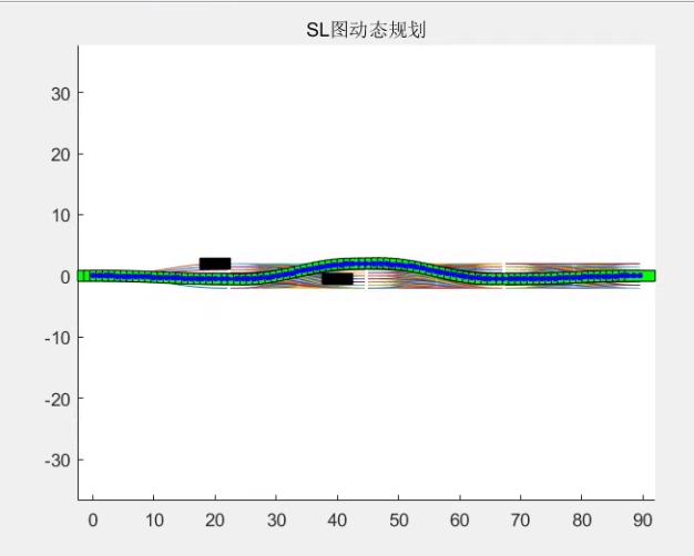
基于动态规划的路径规划和速度规划 EMplanner注释版本matlab代码

基于动态规划的路径规划和速度规划
EMplanner注释版本matlab代码
该算法使用dp动态规划进行了轨迹规划，过程中没有像apollo的EMplanner一样还使用了QP进行了轨迹规划
内容:matlab m代码 详细说明文档 有代码讲解

基于动态规划（Dynamic Programming, DP）的路径规划和速度规划是一种高效的方法，广泛应用于自动驾驶领域。以下是一个详细的实现方案，包括 EMplanner 的注释版本 MATLAB 代码、详细说明文档以及代码讲解。

---

1. 动态规划 (DP) 算法概述

动态规划是一种自底向上的优化算法，适用于求解多阶段决策问题。在自动驾驶中，DP 可用于路径规划和速度规划：

• 路径规划：通过构建代价函数，寻找从起点到终点的最优路径。
• 速度规划：在已知路径的基础上，优化车辆的速度曲线以满足舒适性和安全性要求。

---

2. 算法流程

2.1 路径规划

1. 离散化搜索空间：
   • 将地图划分为网格（或采样点），每个网格点表示一个状态（如位置、方向）。
2. 构建代价函数：
   • 代价函数通常包括距离代价、障碍物代价等。
3. 递推公式：
   • 使用 Bellman 方程递推计算每个状态的最小代价：
     [
     C(i) = \min_{j \in \text{predecessors}(i)} \left[ C(j) + \text{cost}(j \to i) \right]
     ]
4. 回溯路径：
   • 从终点回溯到起点，生成最优路径。

2.2 速度规划

1. 速度离散化：
   • 在路径上对速度进行离散化采样。
2. 约束条件：
   • 加速度、加加速度、碰撞避免等。
3. 递推公式：
   • 类似路径规划，使用 Bellman 方程计算最小代价。

---

3. MATLAB 实现

3.1 路径规划代码

function [path, cost_map] = dp_path_planning(obstacle_map, start_point, end_point, grid_size)
    % 输入参数：
    % obstacle_map: 障碍物地图（二维矩阵，1 表示障碍物）
    % start_point: 起点 [x_start, y_start]
    % end_point: 终点 [x_end, y_end]
    % grid_size: 网格大小

    % 初始化
    [rows, cols] = size(obstacle_map);
    cost_map = inf(rows, cols); % 代价矩阵
    cost_map(start_point(2), start_point(1)) = 0; % 起点代价为 0
    parent_map = zeros(rows, cols, 2); % 父节点记录

    % 动态规划递推
    for i = 1:rows
        for j = 1:cols
            if obstacle_map(i, j) == 1
                continue; % 跳过障碍物
            end
            neighbors = get_neighbors([i, j], rows, cols); % 获取邻居
            for k = 1:size(neighbors, 1)
                ni = neighbors(k, 1);
                nj = neighbors(k, 2);
                new_cost = cost_map(ni, nj) + compute_cost([ni, nj], [i, j], obstacle_map);
                if new_cost < cost_map(i, j)
                    cost_map(i, j) = new_cost;
                    parent_map(i, j, :) = [ni, nj];
                end
            end
        end
    end

    % 回溯路径
    path = [];
    current_point = end_point;
    while ~isequal(current_point, start_point)
        path = [current_point; path];
        current_point = parent_map(current_point(2), current_point(1), :);
    end
    path = [start_point; path];
end

function neighbors = get_neighbors(point, rows, cols)
    % 获取邻居点
    directions = [-1, 0; 1, 0; 0, -1; 0, 1]; % 上下左右
    neighbors = [];
    for d = 1:size(directions, 1)
        ni = point(1) + directions(d, 1);
        nj = point(2) + directions(d, 2);
        if ni >= 1 && ni <= rows && nj >= 1 && nj <= cols
            neighbors = [neighbors; ni, nj];
        end
    end
end

function cost = compute_cost(p1, p2, obstacle_map)
    % 计算两点间的代价
    distance_cost = norm(p1 - p2);
    obstacle_cost = sum(obstacle_map(min(p1(1), p2(1)):max(p1(1), p2(1)), min(p1(2), p2(2)):max(p1(2), p2(2))));
    cost = distance_cost + 10 * obstacle_cost; % 权重可调
end

---

3.2 速度规划代码

function [speed_profile, cost_speed] = dp_speed_planning(path, max_speed, max_acc, dt)
    % 输入参数：
    % path: 路径点集合
    % max_speed: 最大速度
    % max_acc: 最大加速度
    % dt: 时间步长

    % 初始化
    num_points = size(path, 1);
    speed_map = inf(num_points, max_speed / dt); % 速度代价矩阵
    speed_map(1, :) = 0; % 起点速度代价为 0

    % 动态规划递推
    for i = 1:num_points-1
        for v = 1:max_speed/dt
            for a = -max_acc/dt:max_acc/dt
                new_v = v + a * dt;
                if new_v < 0 || new_v > max_speed/dt
                    continue; % 超出速度范围
                end
                new_cost = speed_map(i, v) + compute_speed_cost(v, new_v, a, dt);
                if new_cost < speed_map(i+1, new_v)
                    speed_map(i+1, new_v) = new_cost;
                end
            end
        end
    end

    % 回溯速度曲线
    speed_profile = [];
    [~, best_v] = min(speed_map(end, :));
    for i = num_points:-1:1
        speed_profile = [best_v * dt; speed_profile];
        [~, best_v] = min(speed_map(i, :));
    end
end

function cost = compute_speed_cost(v, new_v, a, dt)
    % 计算速度代价
    jerk_cost = abs((new_v - v) / dt - a); % 加加速度代价
    comfort_cost = abs(a); % 加速度代价
    cost = 0.1 * jerk_cost + 0.5 * comfort_cost; % 权重可调
end

---

4. 说明文档

4.1 文件结构

• dp_path_planning.m: 路径规划函数。
• dp_speed_planning.m: 速度规划函数。
• main.m: 主程序，调用上述函数并可视化结果。

4.2 参数说明

• obstacle_map: 障碍物地图，1 表示障碍物，0 表示自由空间。
• start_point, end_point: 起点和终点坐标。
• max_speed, max_acc: 最大速度和加速度限制。
• dt: 时间步长。

4.3 输出结果

• path: 规划的路径点集合。
• speed_profile: 每个路径点对应的速度。

---

5. 运行示例

% 示例运行
obstacle_map = [0 0 1 0 0; ...
                0 0 1 0 0; ...
                0 0 0 0 0; ...
                0 0 1 0 0; ...
                0 0 0 0 0];
start_point = [1, 1];
end_point = [5, 5];
grid_size = 1;

[path, cost_map] = dp_path_planning(obstacle_map, start_point, end_point, grid_size);

max_speed = 10; % m/s
max_acc = 2; % m/s^2
dt = 0.1; % s
[speed_profile, cost_speed] = dp_speed_planning(path, max_speed, max_acc, dt);

% 可视化
figure;
subplot(1, 2, 1);
imagesc(obstacle_map);
hold on;
plot(path(:, 2), path(:, 1), 'r', 'LineWidth', 2);
title('Path Planning');

subplot(1, 2, 2);
plot(speed_profile, 'b', 'LineWidth', 2);
title('Speed Profile');
xlabel('Path Point');
ylabel('Speed (m/s)');

---

以上代码和文档提供了一个完整的基于 DP 的路径和速度规划实现方案，适用于自动驾驶场景。