


从纯文本构建知识图谱可能具有挑战性。这通常需要识别重要术语、弄清楚它们之间的关系,并使用自定义代码或机器学习工具来提取这种结构。
LLM 驱动的 KG 流水线
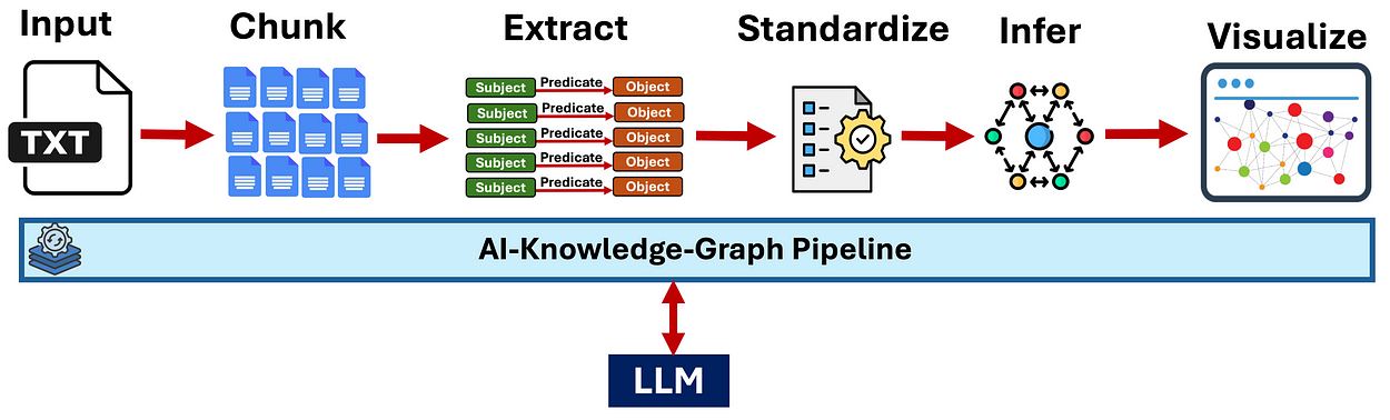
我们将创建一个端到端的 LLM 驱动的流水线,将原始文本自动转换为交互式知识图谱。
所有代码可在以下 GitHub 仓库获取:
GitHub - FareedKhan-dev/KG-Pipeline: 将非结构化数据转换为知识图谱:一个端到端的流水线
目录
搭建环境
什么是知识图谱?
主语 - 谓语 - 宾语(SPO)三元组
配置我们的 LLM 连接
定义我们的输入文本(原始材料)
切分文本:文本切块
LLM 提示词
从 LLM 获取三元组
标准化与去重
使用 NetworkX 创建图
使用 ipycytoscape 创建交互式图
我们接下来可以做什么?
搭建环境
要完成一个好的项目,我们就需要准备工具。我们将使用几个关键的 Python 库来完成任务,先安装它们。
| #Install libraries (run this cell once) pip install openai networkx "ipycytoscape>=1.3.1" ipywidgets pandas |
安装完成后,你可能需要重启 Jupyter 内核或运行时环境以使更改生效。
现在我们已经安装了这些库,让我们将它们导入脚本。
| import openai # 用于与 LLM 交互 import json # 用于解析 LLM 响应 import networkx as nx # 用于创建和管理图数据结构 import ipycytoscape # 用于在笔记本内进行交互式图可视化 import ipywidgets # 用于交互元素 import pandas as pd # 用于以表格形式显示数据 import os # 用于访问环境变量(更安全的 API 密钥存储方式) import math # 用于基本数学运算 import re # 用于基本文本清理(正则表达式) import warnings # 用于抑制潜在的弃用警告 |
现在我们的工具箱已经准备就绪。所有必要的库都已加载到我们的环境中。
什么是知识图谱?
想象一个网络,它就像社交网络一样,但除了人之外,它还连接事实和概念,这基本上就是知识图谱(KG)。它主要有两个部分:
-
节点(或实体):这些是 “事物” —— 例如 “玛丽・居里”“物理学”“巴黎”“诺贝尔奖”。在我们的项目中,我们提取的每个唯一主语或宾语都将变成一个节点。
-
边(或关系):这些是事物之间的连接,展示它们如何相互关联。至关重要的是,这些连接具有意义,通常还有方向。例如:“玛丽・居里” —— 获得 → “诺贝尔奖”。“获得” 这部分是关系,定义了边。
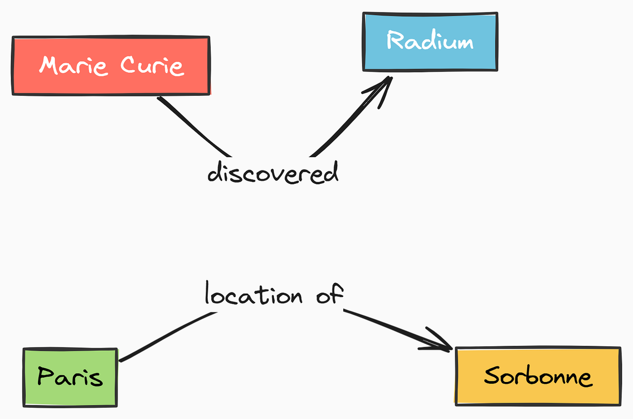
简单的基础信息知识图谱
一个简单图示,显示两个节点(例如 “玛丽・居里” 和 “镭”)通过一个标记为 “发现” 的有向边相连。再添加一个小的集群,如 “巴黎” —— 位置 → “索邦大学”。这可视化了节点 - 边 - 节点的概念。
知识图谱之所以强大,是因为它们以更接近我们思考连接方式的结构组织信息,使我们更容易找到见解,甚至推断出新事实。
主语 - 谓语 - 宾语(SPO)三元组
那么,我们如何从纯文本中获取这些节点和边呢?我们寻找简单的事实陈述,通常以主语 - 谓语 - 宾语(SPO)三元组的形式呈现。
-
主语:事实是关于谁或什么的(例如 “玛丽・居里”),将成为节点。
-
谓语:链接主语和宾语的动作或关系(例如 “发现”),将成为边的标签。
-
宾语:主语相关的事物(例如 “镭”),将成为另一个节点。
示例:句子 “玛丽・居里发现了镭” 完美地分解为三元组:(玛丽・居里,发现,镭)。
这直接转换为我们的图:
(玛丽・居里)-[发现]->(镭)。
LLM 的任务将是阅读文本并为我们识别这些基本的 SPO 事实。
配置我们的 LLM 连接
要使用 LLM,我们需要告诉脚本如何与之通信。这意味着需要提供 API 密钥,有时还需要一个特定的 API 端点(URL)。
我们将使用 NebiusAI LLMs api,但你可以使用 ollama 或其他在 OpenAI 模块下工作的 LLM 提供商。
| # 如果使用标准 OpenAI export OPENAI_API_KEY='your_openai_api_key_here' # 如果使用本地模型,如 Ollama export OPENAI_API_KEY='ollama' # 对于 Ollama,可以是任何非空字符串 export OPENAI_API_BASE='http://localhost:11434/v1' # 如果使用其他提供商,如 Nebius AI export OPENAI_API_KEY='your_provider_api_key_here' export OPENAI_API_BASE='https://api.studio.nebius.com/v1/' # 示例 URL |
首先,让我们指定要使用的 LLM 模型。这取决于你的 API 密钥和端点可用的模型。
| llm_model_name = "deepseek-ai/DeepSeek-V3" # <-- *** 根据你的模型进行更改 *** |
好的,我们已经记录了目标模型。现在,让我们从之前(希望你已经设置好了)设置的环境变量中获取 API 密钥和基础 URL。
| api_key = os.getenv("OPENAI_API_KEY") base_url = os.getenv("OPENAI_API_BASE") # 如果未设置(例如对于标准 OpenAI),则为 None |
客户端已准备好与 LLM 通信。
最后,让我们设置一些控制 LLM 行为的参数:
-
温度:控制随机性。较低的温度意味着更专注、更确定性的输出(适合事实提取!)。我们将温度设置为 0.0 以获得最大可预测性。
-
最大令牌数:限制 LLM 响应的长度。
| llm_temperature = 0.0 # 较低的温度可获得更确定性的、事实性输出。提取时 0.0 最佳。 llm_max_tokens = 4096 # LLM 响应的最大令牌数(根据模型限制进行调整) |
定义我们的输入文本(原始材料)
现在,我们需要想要转换为知识图谱的文本。我们将使用玛丽・居里的传记作为示例。
| unstructured_text = """ Marie Curie, born Maria Skłodowska in Warsaw, Poland, was a pioneering physicist and chemist. She conducted groundbreaking research on radioactivity. Together with her husband, Pierre Curie, she discovered the elements polonium and radium. Marie Curie was the first woman to win a Nobel Prize, the first person and only woman to win the Nobel Prize twice, and the only person to win the Nobel Prize in two different scientific fields. She won the Nobel Prize in Physics in 1903 with Pierre Curie and Henri Becquerel. Later, she won the Nobel Prize in Chemistry in 1911 for her work on radium and polonium. During World War I, she developed mobile radiography units, known as 'petites Curies', to provide X-ray services to field hospitals. Marie Curie died in 1934 from aplastic anemia, likely caused by her long-term exposure to radiation.""" |
让我们打印出来并看看它的长度。
| print("--- 已加载输入文本 ---") print(unstructured_text) print("-" * 25) # 基本统计信息可视化 char_count = len(unstructured_text) word_count = len(unstructured_text.split()) print(f"总字符数:{char_count}") print(f"大约字数:{word_count}") print("-" * 25) |
输出
| --- 已加载输入文本 --- Marie Curie, born Maria Skłodowska in Warsaw, Poland, was a pioneering physicist and chemist. She conducted groundbreaking research on radioactivity. Together with her husband, Pierre Curie, # [... 文本其余部分打印在此处 ...] includes not only her scientific discoveries but also her role in breaking gender barriers in academia and science. ------------------------- 总字符数:1995 大约字数:324 ------------------------- |
所以,我们有关于玛丽・居里的文本,大约 324 个字,对于生产环境来说不太理想,但足以展示知识图谱的构建过程。
切分文本:文本切块
LLM 通常对其一次能处理的文本量(其 “上下文窗口”)有限。
我们的玛丽・居里文本相对较短,但对于较长的文档,我们肯定需要将它们分解为更小的部分,即切块。即使对于这个文本,切块有时也可以帮助 LLM 专注于特定部分。
我们将为切块定义两个参数:
-
切块大小:每个切块中我们想要的最大字数。
-
重叠:一个切块的末尾和下一个切块的开头之间应重叠的字数。这种重叠有助于保留上下文,使事实不会尴尬地在切块之间被切断。
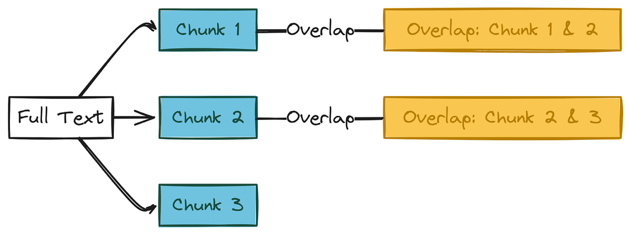
文本切块过程
| # --- 切块配置 --- chunk_size = 150 # 每个切块的字数(根据需要调整) overlap = 30 # 重叠的字数(必须小于切块大小) print(f"切块大小设置为:{chunk_size} 字") print(f"重叠设置为:{overlap} 字") # --- 基本验证 --- if overlap >= chunk_size and chunk_size > 0: print(f"错误:重叠 ({overlap}) 必须小于切块大小 ({chunk_size})。") raise SystemExit("切块配置错误。") else: print("切块配置有效。") |
输出
| 切块大小设置为:150 字 重叠设置为:30 字 切块配置有效。 |
好的,计划是制作 150 字的切块,切块之间重叠 30 字。
首先,我们需要将文本拆分为单独的字。
| words = unstructured_text.split() total_words = len(words) print(f"文本拆分为 {total_words} 个字。") # 可视化前 20 个字 print(f"前 20 个字:{words[:20]}") |
输出
| 文本拆分为 324 个字。 前 20 个字:['Marie', 'Curie,', 'born', 'Maria', 'Skłodowska', 'in', 'Warsaw,', 'Poland,', 'was', 'a', 'pioneering', 'physicist', 'and', 'chemist.', 'She', 'conducted', 'groundbreaking', 'research', 'on', 'radioactivity.'] |
输出确认我们的文本有 324 个字,并显示了前几个字。现在,让我们应用切块逻辑。
我们将逐步遍历字列表,每次获取 chunk_size 个字,然后回退 overlap 个字以开始下一个切块。
| chunks = [] start_index = 0 chunk_number = 1 print(f"开始切块过程...") while start_index < total_words: end_index = min(start_index + chunk_size, total_words) chunk_text = " ".join(words[start_index:end_index]) chunks.append({"text": chunk_text, "chunk_number": chunk_number}) # print(f" 创建切块 {chunk_number}: 字 {start_index} 到 {end_index-1}") # 取消注释以获取详细日志 # 计算下一个切块的起始位置 next_start_index = start_index + chunk_size - overlap # 确保取得进展 if next_start_index <= start_index: if end_index == total_words: break # 已处理最后一部分 next_start_index = start_index + 1 start_index = next_start_index chunk_number += 1 # 安全退出(可选) if chunk_number > total_words: # 简单安全措施 print("警告:切块循环超出总字数,退出。") break print(f"\n文本成功切分为 {len(chunks)} 个切块。") |
输出
| 开始切块过程... 文本成功切分为 3 个切块。 |
太好了!我们的 324 字文本根据我们的大小和重叠设置被分成了 3 个切块。让我们使用 Pandas DataFrame 查看这些切块,了解它们的大小和内容片段。
| print("--- 切块详细信息 ---") if chunks: # 创建 DataFrame 以便更好地可视化 chunks_df = pd.DataFrame(chunks) chunks_df['word_count'] = chunks_df['text'].apply(lambda x: len(x.split())) display(chunks_df[['chunk_number', 'word_count', 'text']]) else: print("未创建切块(文本可能比切块大小短)。") print("-" * 25) |
表格清楚地显示了我们的 3 个切块。注意前两个切块正好是 150 字,最后一个切块包含剩余的 84 个字。完美!现在我们有了可以提供给 LLM 的易于管理的片段。
LLM 提示词
这可能是最重要的部分。能否从 LLM 获得好的结果在很大程度上取决于给出清晰、精确的指令 —— 提示词。
我们需要告诉它我们想要的确切内容(SPO 三元组)以及我们想要的确切格式(特定的 JSON 结构)。
我们将为提示词创建两部分:
-
系统提示词:为 LLM 设置总体角色和上下文(例如,“你是知识图谱提取方面的专家”)。
-
用户提示词:包含特定任务指令和要处理的实际文本切块。
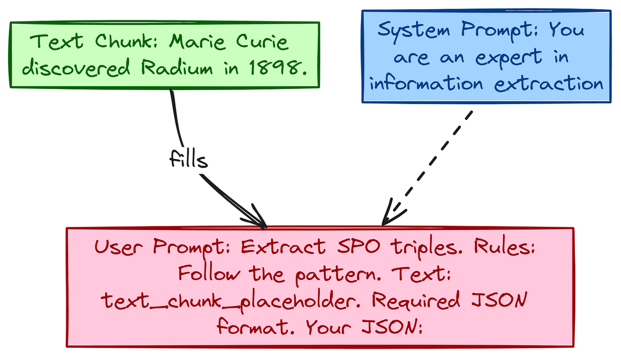
LLM 提示词模板
一个图示,显示两个盒子。盒子 1 标记为 “系统提示词”,包含诸如 “你是专家……” 的文本。
盒子 2 标记为 “用户提示词”,包含诸如 “提取 SPO 三元组…… 规则:…… 文本:{text_chunk}…… 所需 JSON 格式:…… 你的 JSON:” 的文本。
箭头指向用户提示词框中的 {text_chunk} 占位符,表示文本切块数据。
以下是我们在用户提示词中强调的关键规则:
-
提取主语 - 谓语 - 宾语三元组。
-
仅输出一个有效的 JSON 数组 [... ]。元素必须是具有 “主语”“谓语”“宾语” 键的对象。
-
仅输出 JSON。不要在 JSON 数组前后添加任何文字(例如,不要写 “这是 JSON:” 或解释内容)。不要使用 markdown json ... 标签。
-
谓语保持简洁。将 “谓语” 值保持在 1 - 3 个字(理想情况下为 1 - 2 个字)。使用动词或简短的动词短语(例如 “发现”“出生于”“获奖”)。
-
全部小写。所有 “主语”“谓语” 和 “宾语” 的值必须全部小写。这有助于后续的标准化。
-
代词解析。根据文本上下文将代词(她、他、它、她等)替换为具体的实体名称(例如 “玛丽・居里”)。
-
具体化。如果文本中提到了具体细节(例如 “物理学诺贝尔奖” 而不仅仅是 “诺贝尔奖”),则应捕捉这些具体细节。
-
尽力捕捉所有不同的事实。
让我们在 Python 中定义这些提示词。
| # --- 系统提示词:为 LLM 设置上下文 / 角色 --- extraction_system_prompt = """ 你是一位专门从事知识图谱提取的人工智能专家。 你的任务是从给定文本中识别并提取事实性的主语 - 谓语 - 宾语(SPO)三元组。 专注于准确性,并严格遵循用户提示词中请求的 JSON 输出格式。 提取核心实体及其最直接的关系。""" # --- 用户提示词模板:包含具体指令和文本 --- extraction_user_prompt_template = """ 请从以下文本中提取主语 - 谓语 - 宾语(S-P-O)三元组。 ** 非常重要的规则:** 1. **输出格式:** 仅回复一个有效的 JSON 数组。每个元素必须是具有 “主语”“谓语”“宾语” 键的对象。 2. **仅 JSON:** 不要在 JSON 数组前后添加任何文字(例如,不要写 “这是 JSON:” 或解释内容)。不要使用 markdown ```json ... ``` 标签。 3. **简洁的谓语:** 将 “谓语” 值保持在 1 - 3 个字(理想情况下为 1 - 2 个字)。使用动词或简短的动词短语(例如 “发现”“出生于”“获奖”)。 4. **全部小写:** “主语”“谓语” 和 “宾语” 的所有值必须全部小写。 5. **代词解析:** 根据文本上下文将代词(她、他、它、她等)替换为具体的实体名称(例如 “玛丽・居里”)。 6. **具体化:** 捕捉具体细节(例如,如果提到 “物理学诺贝尔奖” 而不仅仅是 “诺贝尔奖”)。 7. **完整性:** 提取所有提到的不同事实。 **要处理的文本:** ```text {text_chunk} """ |
让我们打印出来,仅为了双重检查它们是否正确,包括插入第一个文本切块时用户提示词的示例。
| print("--- 系统提示词 ---") print(extraction_system_prompt) print("\n" + "-" * 25 + "\n") print("--- 用户提示词模板(结构) ---") # 显示结构,替换占位符以便清晰 print(extraction_user_prompt_template.replace("{text_chunk}", "[... 文本切块放在这里 ...]")) print("\n" + "-" * 25 + "\n") # 显示实际将用于第一个切块的提示词示例 print("--- 第一个切块的示例填充用户提示词 ---") if chunks: example_filled_prompt = extraction_user_prompt_template.format(text_chunk=chunks[0]['text']) # 为了简洁,显示有限部分 print(example_filled_prompt[:600] + "\n[... 其余切块文本 ...]\n" + example_filled_prompt[-200:]) else: print("没有可用切块来创建示例填充提示词。") print("\n" + "-" * 25) |
输出
| 你是一位专门从事知识图谱提取的人工智能专家。 你的任务是从给定文本中识别并提取事实性的主语 - 谓语 - 宾语(SPO)三元组。 专注于准确性,并严格遵循用户提示词中请求的 JSON 输出格式。 提取核心实体及其最直接的关系。 ------------------------- --- 用户提示词模板(结构) --- 请从以下文本中提取主语 - 谓语 - 宾语(S-P-O)三元组。 ** 非常重要的规则:** # [... 规则打印在此处 ...] **要处理的文本:** ```text [... 文本切块放在这里 ...] |
看起来不错!提示词清楚地说明了任务和严格的格式要求。我们已准备好将它们发送给 LLM。
从 LLM 获取三元组
现在是令人兴奋的部分!我们将循环遍历每个文本切块,使用切块的文本格式化用户提示词,通过 API 将系统提示词和用户提示词发送给 LLM,然后尝试解析返回的 JSON 响应。 我们会记录成功的提取结果以及任何失败的片段。
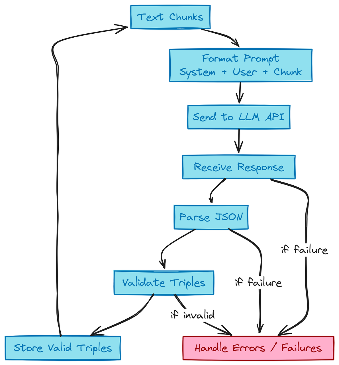
LLM 流程中的三元组
它展示了一个循环。从 “文本片段” 开始。箭头指向 “格式化提示(系统 + 用户 + 片段)”。箭头指向 “发送至 LLM API”。箭头指向 “接收响应”。箭头指向 “解析 JSON”。箭头指向 “验证三元组”。箭头指向 “存储有效三元组”。 箭头回到开始处以处理下一个片段。在旁边包含一个小框用于 “处理错误 / 失败”。
让我们初始化我们的存储列表。
| #Initialize lists to store results and failures all_extracted_triples = [] failed_chunks = [] print(f"Starting triple extraction from {len(chunks)} chunks using model '{llm_model_name}'...") #We will process chunks one by one in the following cells. #### OUTPUT #### Starting triple extraction from 3 chunks using model 'deepseek-ai/DeepSeek-V3'... |
好的,让我们处理第一个片段(记住,完整的笔记本会遍历所有片段,但为了清晰起见,这里我们只展示一个片段的详细步骤)。
| chunk_index = 0 # Process first chunk only if chunk_index < len(chunks): chunk = chunks[chunk_index] prompt = extraction_user_prompt_template.format(text_chunk=chunk['text']) try: # Call LLM with system + user prompt res = client.chat.completions.create( model=llm_model_name, messages=[{"role": "system", "content": extraction_system_prompt}, {"role": "user", "content": prompt}], temperature=llm_temperature, max_tokens=llm_max_tokens, response_format={"type": "json_object"}, ) raw = res.choices[0].message.content.strip() except Exception as e: failed_chunks.append({'chunk_number': chunk['chunk_number'], 'error': str(e), 'response': ''}) print("LLM call failed."); exit() # Try JSON parsing directly or via regex fallback try: data = json.loads(raw) if isinstance(data, dict): data = next((v for v in data.values() if isinstance(v, list)), []) except: match = re.search(r'(\[.*\])', raw, re.DOTALL) data = json.loads(match.group(1)) if match else [] # Validate and store triples triples = [dict(t, chunk=chunk['chunk_number']) for t in data if isinstance(t, dict) and all(k in t and isinstance(t[k], str) for k in ['subject', 'predicate', 'object'])] if triples: all_extracted_triples.extend(triples) else: failed_chunks.append({'chunk_number': chunk['chunk_number'], 'error': 'No valid triples', 'response': raw}) print("Done.") |
当我们运行上述循环时,它将开始提取实体和其他将用于为我们创建知识图谱的元素。 这就是单次试验(一个片段处理)的样子。
--- Processing Chunk 1/3 ---
1. Formatting User Prompt...
2. Sending request to LLM...
   LLM response received.
3. Extracting raw response content...
--- Raw LLM Output (Chunk 1) ---
[
  { "subject": "marie curie", "predicate": "born as", "object": "maria skłodowska" },
  { "subject": "marie curie", "predicate": "born in", "object": "warsaw, poland" },
  { "subject": "marie curie", "predicate": "was", "object": "physicist" },
  # [... more raw triples ...]
  { "subject": "marie curie", "predicate": "born to", "object": "family of teachers" }
]
--------------------
4. Attempting to parse JSON from response...
   Successfully parsed JSON list directly.
--- Parsed JSON Data (Chunk 1) ---
[
  {
    "subject": "marie curie",
    "predicate": "born as",
    "object": "maria sk\u0142odowska"
  },
  # [... more parsed triples ...]
  {
    "subject": "marie curie",
    "predicate": "born to",
    "object": "family of teachers"
  }
]
--------------------
5. Validating structure and extracting triples...
   Found 18 valid triples in this chunk.
--- Valid Triples Extracted (Chunk 1) ---
        subject   predicate                                                object  chunk
0   marie curie     born as                                      maria skłodowska      1
1   marie curie     born in                                        warsaw, poland      1
2   marie curie         was                                             physicist      1
# [... more triples displayed in DataFrame ...]
17  marie curie     born to                                    family of teachers      1
--------------------
--- Running Total Triples Extracted: 18 ---
--- Failed Chunks So Far: 0 ---

Finished processing this chunk.
我们发送了第一个片段,得到了响应,并成功将其解析为 JSON。原始输出显示 LLM 相当好地遵循了我们的指令,提供了一个字典列表。然后我们验证了这些字典并以表格形式整齐地展示出来 —— 仅从第一个片段就提取了 18 个事实! (记住:上面的代码仅运行于片段 1。完整的运行会处理所有片段,累积更多的三元组。) 让我们总结一下尝试所有片段后的总体结果(基于完整笔记本运行)。
# --- Summary of Extraction (Reflecting state after the single chunk demo / or full run) ---
print(f"\n--- Overall Extraction Summary ---\n")
print(f"Total chunks defined: {len(chunks)}\")\n"
# Assuming full run for summary logic
processed_chunks = len(chunks) # Approximation if loop isn't run fully
print(f"Chunks processed (attempted): {processed_chunks}") # Chunks we looped through
print(f"Total valid triples extracted across all processed chunks: {len(all_extracted_triples)}")
print(f"Number of chunks that failed API call or parsing: {len(failed_chunks)}")

if failed_chunks:
    print("\nDetails of Failed Chunks:")
    failed_df = pd.DataFrame(failed_chunks)
    display(failed_df[['chunk_number', 'error']]) # Display failed chunks neatly
    # for failure in failed_chunks:
    #     print(f"  Chunk {failure['chunk_number']}: Error: {failure['error']}")
print("-" * 25)

# Display all extracted triples using Pandas
print("\n--- All Extracted Triples (Before Normalization) ---")
if all_extracted_triples:
    all_triples_df = pd.DataFrame(all_extracted_triples)
    display(all_triples_df)
else:
    print("No triples were successfully extracted.")
print("-" * 25)
输出结果:
--- Overall Extraction Summary ---
Total chunks defined: 3
Chunks processed (attempted): 3
Total valid triples extracted across all processed chunks: 45  # <--- Example total
Number of chunks that failed API call or parsing: 0
-------------------------

--- All Extracted Triples (Before Normalization) ---
        subject      predicate                        object  chunk
0   marie curie        born as              maria skłodowska      1
1   marie curie        born in                warsaw, poland      1
# [... many more triples from all chunks ...]
44  marie curie  had daughters                          irène      3
-------------------------
好的,在处理完所有片段(完整运行后),我们得到了一个包含 LLM 找到的所有三元组的组合列表。这是一个不错的开始,但你可能会注意到一些潜在的重叠或细微差异。是时候清理一下了!
规范化与去重
LLM 的原始输出很棒,但通常需要一些润色。我们将执行几个简单的清理步骤:
-
规范化:修剪主体、谓词和客体开头或结尾的多余空格。我们已经要求 LLM 使用小写,但为以防万一,这里我们会再次强制执行。
-
过滤:移除在修剪后任一部分为空的三元组(例如,如果 LLM 返回了空格 " ")。
-
去重:移除同一(主体,谓词,客体)事实的精确副本,这些副本可能从重叠的片段或文本中的不同表述中提取出来。
让我们初始化这个过程。
# Initialize lists and tracking variables
normalized_triples = []
seen_triples = set() # Tracks (subject, predicate, object) tuples
original_count = len(all_extracted_triples)
empty_removed_count = 0
duplicates_removed_count = 0

print(f"Starting normalization and de-duplication of {original_count} triples...")

#### OUTPUT ####
Starting normalization and de-duplication of 45 triples... # <--- Example total
现在,我们将遍历原始的 all_extracted_triples,应用清理步骤,并仅保留唯一且有效的三元组。
我们将打印前几个转换以展示发生了什么。
print("Processing triples (showing first 5):")

for i, t in enumerate(all_extracted_triples):
    s, p, o = [t.get(k, '').strip().lower() if isinstance(t.get(k), str) else '' for k in ['subject', 'predicate', 'object']]
    p = re.sub(r'\s+', ' ', p)

    if all([s, p, o]):
        key = (s, p, o)
        if key not in seen_triples:
            normalized_triples.append({'subject': s, 'predicate': p, 'object': o, 'source_chunk': t.get('chunk', '?')})
            seen_triples.add(key)
            if i < 5:
                print(f"\n#{i+1}: {key}\nStatus: Kept")
        else:
            duplicates_removed_count += 1
            if i < 5: print(f"\n#{i+1}: Duplicate - Skipped")
    else:
        empty_removed_count += 1
        if i < 5: print(f"\n#{i+1}: Invalid - Skipped")

print(f"\nDone. Total: {len(all_extracted_triples)}, Kept: {len(normalized_triples)}, Duplicates: {duplicates_removed_count}, Empty: {empty_removed_count}")
我们开始循环生成三元组,以下是结果。
Processing triples for normalization (showing first 5 examples):

--- Example 1 ---
Original Triple (Chunk 1): {'subject': 'marie curie', 'predicate': 'born as', 'object': 'maria skłodowska', 'chunk': 1}
Normalized: SUB='marie curie', PRED='born as', OBJ='maria skłodowska'
Status: Kept (New Unique Triple)

--- Example 2 ---
Original Triple (Chunk 1): {'subject': 'marie curie', 'predicate': 'born in', 'object': 'warsaw, poland', 'chunk': 1}
Normalized: SUB='marie curie', PRED='born in', OBJ='warsaw, poland'
Status: Kept (New Unique Triple)

... Finished processing 45 triples. # <--- Example total
从最初的几个示例可以看出,该过程会检查每个三元组。如果它是有效的(清理后不为空),并且我们以前没有遇到过这个确切的事实,我们就保留它。
让我们总结一下我们开始时的三元组数量、移除了多少,以及显示最终的干净列表。
# --- Summary of Normalization ---
print(f"\n--- Normalization & De-duplication Summary ---\n")
print(f"Original extracted triple count: {original_count}\")\n"
print(f"Triples removed (empty/invalid components): {empty_removed_count}\")\n"
print(f"Duplicate triples removed: {duplicates_removed_count}\")\n"
final_count = len(normalized_triples)
print(f"Final unique, normalized triple count: {final_count}\")\n"
print("-" * 25)

# Display a sample of normalized triples using Pandas
print("\n--- Final Normalized Triples ---")
if normalized_triples:
    normalized_df = pd.DataFrame(normalized_triples)
    display(normalized_df)
else:
    print("No valid triples remain after normalization.")
print("-" * 25)


#### OUTPUT ####
--- Normalization & De-duplication Summary ---
Original extracted triple count: 45
Triples removed (empty/invalid components): 0
Duplicate triples removed: 3  # <--- Example: some duplicates found
Final unique, normalized triple count: 42 # <--- Example final count
-------------------------

--- Final Normalized Triples ---
        subject         predicate                     object source_chunk
0   marie curie           born as           maria skłodowska            1
1   marie curie           born in             warsaw, poland            1
# [... only unique, clean triples displayed ...]
41  marie curie  had daughter named                      eve            3
-------------------------
使用 NetworkX 创建图
是时候组装我们的知识图谱了!我们将使用 networkx 库创建一个有向图(DiGraph)。以下是我们的干净三元组如何映射到图:
-
每个唯一的主体成为一个节点。
-
每个唯一的客体成为一个节点。
-
每个三元组(主体,谓词,客体)成为从主体节点到客体节点的有向边,谓词作为边的标签。
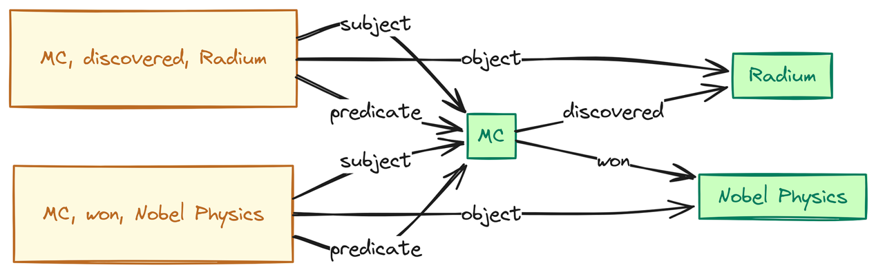
图的构建方式
左侧显示 2-3 个 SPO 三元组(例如,(MC,发现,镭),(MC,获得,诺贝尔物理学奖))。右侧显示对应的图元素: “MC”、“镭”、“诺贝尔物理学奖” 的节点。“MC” 到 “镭” 的边标记为 “发现”。“MC” 到 “诺贝尔物理学奖” 的边标记为 “获得”。使用箭头显示三元组组件到图元素的映射。
首先,让我们创建一个空的图对象。
# Create an empty directed graph
knowledge_graph = nx.DiGraph()

print("Initialized an empty NetworkX DiGraph.")
# Visualize the initial empty graph state
print("--- Initial Graph Info ---")
try:
    # Try the newer method first
    print(nx.info(knowledge_graph))
except AttributeError:
    # Fallback for different NetworkX versions
    print(f"Type: {type(knowledge_graph).__name__}")
    print(f"Number of nodes: {knowledge_graph.number_of_nodes()}")
    print(f"Number of edges: {knowledge_graph.number_of_edges()}")
print("-" * 25)
我们的图目前是空的,正如预期。
现在,我们将遍历我们的 normalized_triples 并将每个三元组作为一条边(及其对应的节点)添加到图中。
我们将定期打印更新以展示图的增长。
print("Adding triples to the NetworkX graph...")

added_edges_count = 0
update_interval = 10 # How often to print graph info update

if not normalized_triples:
    print("Warning: No normalized triples to add to the graph.")
else:
    for i, triple in enumerate(normalized_triples):
        subject_node = triple['subject']
        object_node = triple['object']
        predicate_label = triple['predicate']

        # Nodes are added automatically when adding edges, but explicit calls are fine too
        # knowledge_graph.add_node(subject_node)
        # knowledge_graph.add_node(object_node)

        # Add the directed edge with the predicate as a 'label' attribute
        knowledge_graph.add_edge(subject_node, object_node, label=predicate_label)
        added_edges_count += 1

        # --- Visualize Graph Growth ---
        if (i + 1) % update_interval == 0 or (i + 1) == len(normalized_triples):
            print(f"\n--- Graph Info after adding Triple #{i+1} --- ({subject_node} -> {object_node})")
            try:
                # Try the newer method first
                print(nx.info(knowledge_graph))
            except AttributeError:
                # Fallback for different NetworkX versions
                print(f"Type: {type(knowledge_graph).__name__}")
                print(f"Number of nodes: {knowledge_graph.number_of_nodes()}")
                print(f"Number of edges: {knowledge_graph.number_of_edges()}")
            # For very large graphs, printing info too often can be slow. Adjust interval.

print(f"\nFinished adding triples. Processed {added_edges_count} edges.")


#### OUTPUT ####
Adding triples to the NetworkX graph...

--- Graph Info after adding Triple #10 --- (marie curie -> only woman to win nobel prize twice)
Type: DiGraph
Number of nodes: 11
Number of edges: 10

--- Graph Info after adding Triple #20 --- (pierre curie -> was professor of physics)
Type: DiGraph
Number of nodes: 24
Number of edges: 20
我们遍历了干净的三元组,为每一个添加了一条边到我们的 networkx 图中。
输出显示图在节点和边上稳步增长。
让我们查看最终的统计信息,并查看我们构建的图中的一些示例节点和边。
# --- Final Graph Statistics ---
num_nodes = knowledge_graph.number_of_nodes()
num_edges = knowledge_graph.number_of_edges()

print(f"\n--- Final NetworkX Graph Summary ---\n")
print(f"Total unique nodes (entities): {num_nodes}")
print(f"Total unique edges (relationships): {num_edges}")

if num_edges != added_edges_count and isinstance(knowledge_graph, nx.DiGraph):
     print(f"Note: Added {added_edges_count} edges, but graph has {num_edges}. DiGraph overwrites edges with same source/target. Use MultiDiGraph if multiple edges needed.")

if num_nodes > 0:
    try:
       density = nx.density(knowledge_graph)
       print(f"Graph density: {density:.4f}") # How connected the graph is
       if nx.is_weakly_connected(knowledge_graph): # Can you reach any node from any other, ignoring edge direction?
           print("The graph is weakly connected (all nodes reachable ignoring direction).")
       else:
           num_components = nx.number_weakly_connected_components(knowledge_graph)
           print(f"The graph has {num_components} weakly connected components.")
    except Exception as e:
        print(f"Could not calculate some graph metrics: {e}") # Handle potential errors on empty/small graphs
else:
    print("Graph is empty, cannot calculate metrics.")
print("-" * 25)

# --- Sample Nodes ---
print("\n--- Sample Nodes (First 10) ---")
if num_nodes > 0:
    nodes_sample = list(knowledge_graph.nodes())[:10]
    display(pd.DataFrame(nodes_sample, columns=['Node Sample']))
else:
    print("Graph has no nodes.")

# --- Sample Edges ---
print("\n--- Sample Edges (First 10 with Labels) ---")
if num_edges > 0:
    edges_sample = []
    for u, v, data in list(knowledge_graph.edges(data=True))[:10]:
        edges_sample.append({'Source': u, 'Target': v, 'Label': data.get('label', 'N/A')})
    display(pd.DataFrame(edges_sample))
else:
    print("Graph has no edges.")
print("-" * 25)
我们已成功使用 networkx 在内存中构建了图结构。我们可以看到唯一实体(节点)和关系(边)的总数,并初步了解它们应该是什么样的。
使用 ipycytoscape 创建交互式图
现在到了真正酷的部分,我们可以看到我们的图了!我们将使用 ipycytoscape 在笔记本中创建一个交互式可视化。
首先,快速检查一下我们是否有这样一个图可以进行可视化。
print("Preparing interactive visualization...")

# --- Check Graph Validity for Visualization ---
can_visualize = False
if 'knowledge_graph' not in locals() or not isinstance(knowledge_graph, nx.Graph):
    print("Error: 'knowledge_graph' not found or is not a NetworkX graph.")
elif knowledge_graph.number_of_nodes() == 0:
    print("NetworkX Graph is empty. Cannot visualize.")
else:
    print(f"Graph seems valid for visualization ({knowledge_graph.number_of_nodes()} nodes, {knowledge_graph.number_of_edges()} edges).")
    can_visualize = True

#### OUTPUT ####
Preparing interactive visualization...
Graph seems valid for visualization (35 nodes, 42 edges).
ipycytoscape 需要图数据以特定的 JSON 格式(节点和边的字典列表)提供。
现在我们将转换我们的 networkx 图数据,还将计算节点度(每个节点有多少连接),以便稍后调整节点大小。
cytoscape_nodes = []
cytoscape_edges = []

if can_visualize:
    print("Converting nodes...")
    # Calculate degrees for node sizing
    node_degrees = dict(knowledge_graph.degree())
    max_degree = max(node_degrees.values()) if node_degrees else 1

    for node_id in knowledge_graph.nodes():
        degree = node_degrees.get(node_id, 0)
        # Simple scaling for node size (adjust logic as needed)
        node_size = 15 + (degree / max_degree) * 50 if max_degree > 0 else 15

        cytoscape_nodes.append({
            'data': {
                'id': str(node_id), # ID must be string
                'label': str(node_id).replace(' ', '\n'), # Display label (wrap spaces)
                'degree': degree,
                'size': node_size, # Store size for styling
                'tooltip_text': f"Entity: {str(node_id)}\nDegree: {degree}" # Tooltip on hover
            }
        })
    print(f"Converted {len(cytoscape_nodes)} nodes.")

    print("Converting edges...")
    edge_count = 0
    for u, v, data in knowledge_graph.edges(data=True):
        edge_id = f"edge_{edge_count}" # Unique edge ID
        predicate_label = data.get('label', '')
        cytoscape_edges.append({
            'data': {
                'id': edge_id,
                'source': str(u),
                'target': str(v),
                'label': predicate_label, # Label on edge
                'tooltip_text': f"Relationship: {predicate_label}" # Tooltip on hover
            }
        })
        edge_count += 1
    print(f"Converted {len(cytoscape_edges)} edges.")

    # Combine into the final structure
    cytoscape_graph_data = {'nodes': cytoscape_nodes, 'edges': cytoscape_edges}

    # Visualize the converted structure (first few nodes/edges)
    print("\n--- Sample Cytoscape Node Data (First 2) ---")
    print(json.dumps(cytoscape_graph_data['nodes'][:2], indent=2))
    print("\n--- Sample Cytoscape Edge Data (First 2) ---")
    print(json.dumps(cytoscape_graph_data['edges'][:2], indent=2))
    print("-" * 25)
else:
     print("Skipping data conversion as graph is not valid for visualization.")
     cytoscape_graph_data = {'nodes': [], 'edges': []}
转换已完成。我们的节点和边已正确格式化为 ipycytoscape 提供的格式,包括经计算的大小和有用的工具提示。 让我们创建实际的控件对象,并将我们的图数据加载到其中。 我们可以使用类似于 CSS 的样式语法来控制节点和边的外观。让我们定义一个漂亮、多彩且交互式的样式,我们将根据节点的度来调整节点大小,在悬停 / 选择时更改颜色,并标记边。 让我们渲染控件。您应该在下面这个单元格的输出中看到交互式知识图。
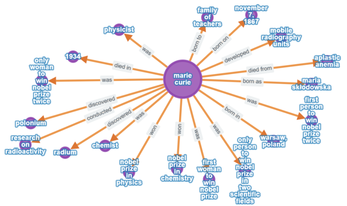
我们的 KG 图
好的,这里是关于知识图的要点:
-
中心实体:marie curie 是中心的主要节点。
-
关系:橙色箭头(边)显示从 marie curie 出发的连接。
-
谓词标签:边上的文字(例如,发现、获得、是)定义了关系。
-
连接实体:箭头末端的节点是对象或相关实体(例如,镭、钋、物理学家)。
-
SPO 三元组:每个箭头代表一个由 LLM 提取的(主体,谓词,客体)事实。
-
视觉摘要:该图提供了关于 marie curie 的事实的快速、结构化概览。
-
图结构:它是围绕 marie curie 的中心辐射风格。
接下来我们可以做什么?
这个流程是一个很好的起点,但总有改进和探索的空间:
-
错误处理:通过重试或更好的处理方式,使 LLM 调用更加健壮,即使某个片段始终失败。
-
高级规范化:超越简单的字符串匹配。实现实体链接(将 “Marie Curie” 和 “M. Curie” 连接到同一个现实世界实体 ID)或关系聚类(将类似的谓词分组,如 “出生于” 和 “生于”)。
-
提示工程:实验!尝试不同的 LLM 模型,调整提示指令,更改温度参数,看看结果如何变化。
-
评估:提取的三元组有多好?实现方法来衡量精度(提取的事实是否正确?)和召回率(我们是否找到了所有事实?)。
-
更丰富的可视化:为不同类型的节点(人物、地点、概念)使用不同的颜色或形状。在可视化中添加更多的交互功能或直接添加图分析结果。
-
图分析:利用 networkx 的强大功能来查找最重要的节点(中心性)、发现实体之间的路径,或识别图中的社区。
-
持久化:保存你的图!将提取的三元组或图结构存储在专用的图数据库(如 Neo4j)中,以便进行更大的项目和更复杂的查询。


 被折叠的 条评论
为什么被折叠?
被折叠的 条评论
为什么被折叠?
 到【灌水乐园】发言


