


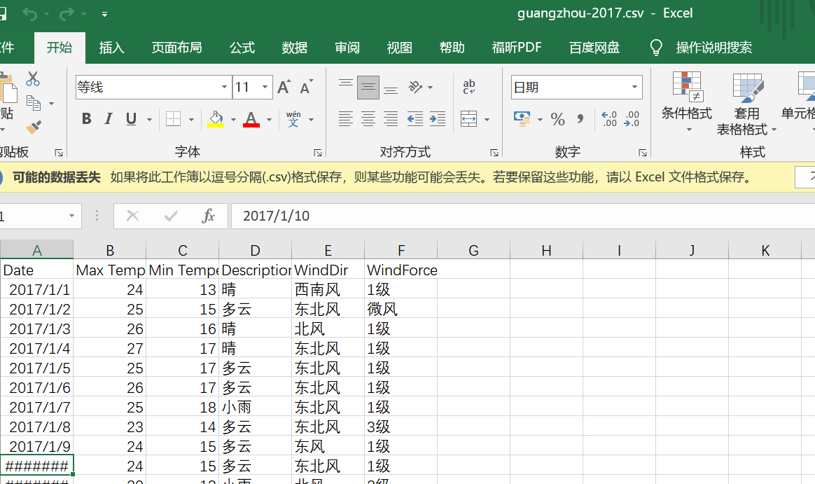
csv文件格式
csv文件格式的本质是一种以文本存储的表格数据(使用excel可以读写csv文件)。
import csv

filename = 'guangzhou-2017.csv'
# 打开文件
with open(filename) as f:
    # 创建cvs文件读取器
    reader = csv.reader(f)
    # 读取第一行,这行是表头数据。
    header_row = next(reader)
    print(header_row)
    # 读取第二行,这行是真正的数据。
    first_row = next(reader)
    print(first_row)
import csv
from datetime import datetime
from matplotlib import pyplot as plt
filename = 'guangzhou-2017.csv'
# 打开文件
with open(filename) as f:
# 创建cvs文件读取器
reader = csv.reader(f)
# 读取第一行,这行是表头数据。
header_row = next(reader)
print(header_row)
# 定义读取起始日期
start_date = datetime(2017, 6, 30)
# 定义结束日期
end_date = datetime(2017, 8, 1)
# 定义3个list列表作为展示的数据
dates, highs, lows = [], [], []
for row in reader:
# 将第一列的值格式化为日期
d = datetime.strptime(row[0], '%Y-%m-%d')
# 只展示2017年7月的数据
if start_date < d < end_date:
dates.append(d)
highs.append(int(row[1]))
lows.append(int(row[2]))
# 配置图形
fig = plt.figure(dpi=128, figsize=(12, 9))
# 绘制最高气温的折线
plt.plot(dates, highs, c='red', label='最高气温',
alpha=0.5, linewidth = 2.0, linestyle = '-', marker='v')
# 再绘制一条折线
plt.plot(dates, lows, c='blue', label='最低气温',
alpha=0.5, linewidth = 3.0, linestyle = '-.', marker='o')
# 为两个数据的绘图区域填充颜色
plt.fill_between(dates, highs, lows, facecolor='blue', alpha=0.1)
# 设置标题
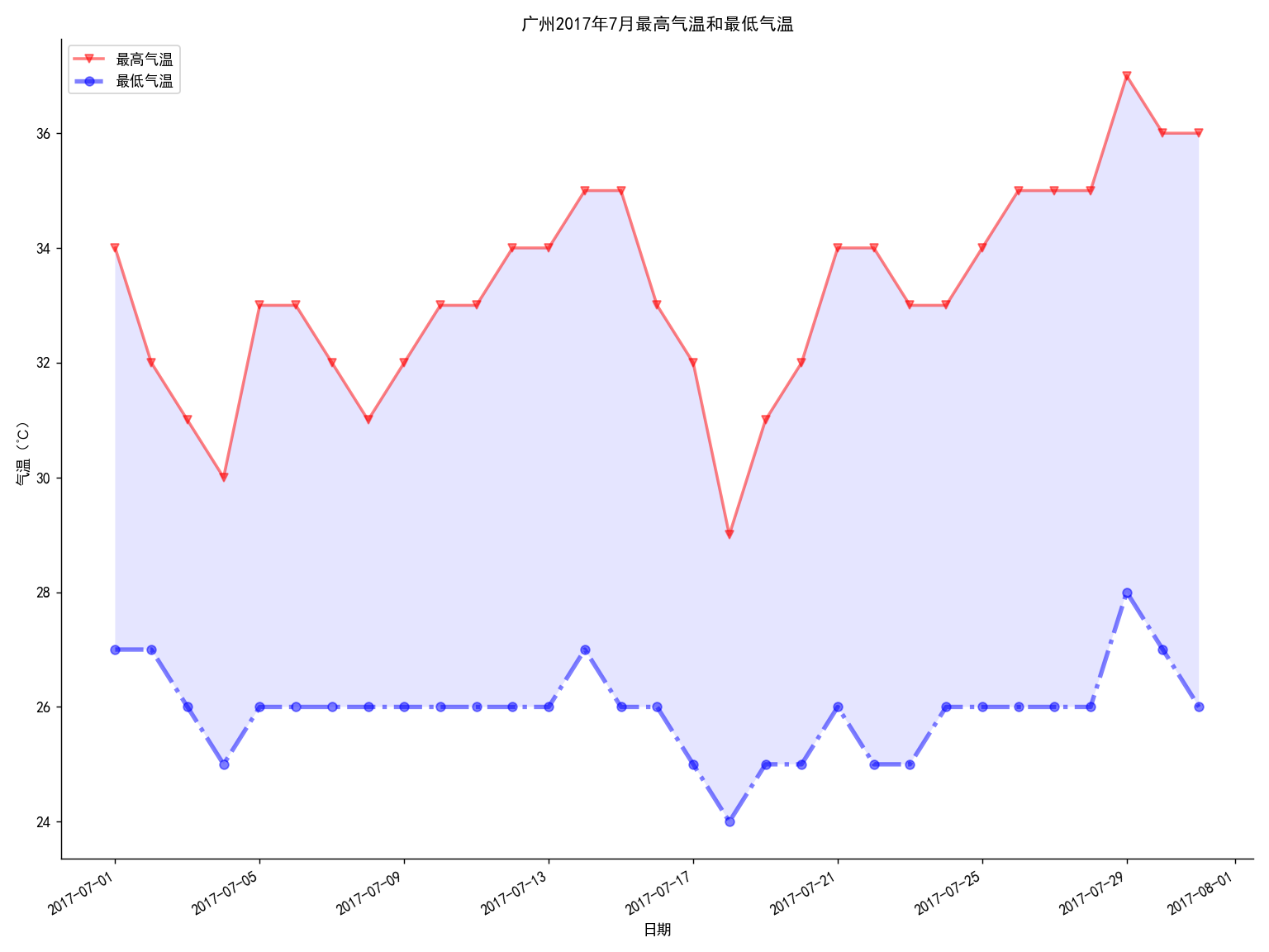
plt.title("广州2017年7月最高气温和最低气温")
# 为两条坐标轴设置名称
plt.xlabel("日期")
# 该方法绘制斜着的日期标签
fig.autofmt_xdate()
plt.ylabel("气温(℃)")
# 显示图例
plt.legend()
ax = plt.gca()
# 设置右边坐标轴线的颜色(设置为none表示不显示)
ax.spines['right'].set_color('none')
# 设置顶部坐标轴线的颜色(设置为none表示不显示)
ax.spines['top'].set_color('none')
plt.rcParams['font.sans-serif'] = ['SimHei']
plt.rcParams['axes.unicode_minus'] = False
plt.show()
import csv
from datetime import datetime
from matplotlib import pyplot as plt
filename = 'guangzhou-2017.csv'
# 打开文件
with open(filename) as f:
# 创建cvs文件读取器
reader = csv.reader(f)
# 读取第一行,这行是表头数据。
header_row = next(reader)
print(header_row)
# 定义读取起始日期
start_date = datetime(2017, 6, 30)
# 定义结束日期
end_date = datetime(2017, 8, 1)
# 定义3个list列表作为展示的数据
dates, highs, lows = [], [], []
for row in reader:
# 将第一列的值格式化为日期
d = datetime.strptime(row[0], '%Y-%m-%d')
# 只展示2017年7月的数据
if start_date < d < end_date:
dates.append(d)
highs.append(int(row[1]))
lows.append(int(row[2]))
# 配置图形
fig = plt.figure(dpi=128, figsize=(12, 9))
# 绘制最高气温的折线
plt.plot(dates, highs, c='red', label='最高气温',
alpha=0.5, linewidth = 2.0, linestyle = '-', marker='v')
# 再绘制一条折线
plt.plot(dates, lows, c='blue', label='最低气温',
alpha=0.5, linewidth = 3.0, linestyle = '-.', marker='o')
# 为两个数据的绘图区域填充颜色
plt.fill_between(dates, highs, lows, facecolor='blue', alpha=0.1)
# 设置标题
plt.title("广州2017年7月最高气温和最低气温")
# 为两条坐标轴设置名称
plt.xlabel("日期")
# 该方法绘制斜着的日期标签
fig.autofmt_xdate()
plt.ylabel("气温(℃)")
# 显示图例
plt.legend()
ax = plt.gca()
# 设置右边坐标轴线的颜色(设置为none表示不显示)
ax.spines['right'].set_color('none')
# 设置顶部坐标轴线的颜色(设置为none表示不显示)
ax.spines['top'].set_color('none')
plt.show()
import csv
import pygal

filename = 'guangzhou-2017.csv'
# 打开文件
with open(filename) as f:
    # 创建cvs文件读取器
    reader = csv.reader(f)
    # 读取第一行,这行是表头数据。
    header_row = next(reader)
    print(header_row)
    # 准备展示的数据
    shades, sunnys, cloudys, rainys = 0, 0, 0, 0
    for row in reader:
        if '阴' in row[3]:
            shades += 1
        elif '晴' in row[3]:
            sunnys += 1
        elif '云' in row[3]:
            cloudys += 1
        elif '雨' in row[3]:
            rainys += 1
        else:
            print(rows[3])
# 创建pygal.Pie对象(饼图)
pie = pygal.Pie()
# 为饼图添加数据
pie.add("阴", shades)
pie.add("晴", sunnys)
pie.add("多云", cloudys)
pie.add("雨", rainys)
pie.title = '2017年广州天气汇总'
# 设置将图例放在底部
pie.legend_at_bottom = True
# 指定将数据图输出到SVG文件中
pie.render_to_file('guangzhou_weather.svg')
JSON数据
import json
from matplotlib import pyplot as plt
import numpy as np
filename = 'gdp_json.json'
# 读取JSON格式的GDP数据
with open(filename) as f:
gpd_list = json.load(f)
# 使用list列表依次保存中国、美国、日本、俄罗斯、加拿大的GDP值
country_gdps = [{}, {}, {}, {}, {}]
country_codes = ['CHN', 'USA', 'JPN', 'RUS', 'CAN']
# 遍历列表的每个元素,每个元素是一个GDP数据项
for gpd_dict in gpd_list:
for i, country_code in enumerate(country_codes):
# 只读取指定国家的数据
if gpd_dict['Country Code'] == country_code:
year = gpd_dict['Year']
# 只读取2001年到2016
if 2017 > year > 2000:
country_gdps[i][year] = gpd_dict['Value']
# 使用list列表依次保存中国、美国、日本、俄罗斯、加拿大的GDP值
country_gdp_list = [[], [], [], [], []]
# 构建时间数据
x_data = range(2001, 2017)
for i in range(len(country_gdp_list)):
for year in x_data:
# 除以1e8,让数值变成以亿为单位
country_gdp_list[i].append(country_gdps[i][year] / 1e8)
bar_width=0.15
fig = plt.figure(dpi=128, figsize=(15, 8))
colors = ['indianred', 'steelblue', 'gold', 'lightpink', 'seagreen']
# 定义国家名称列表
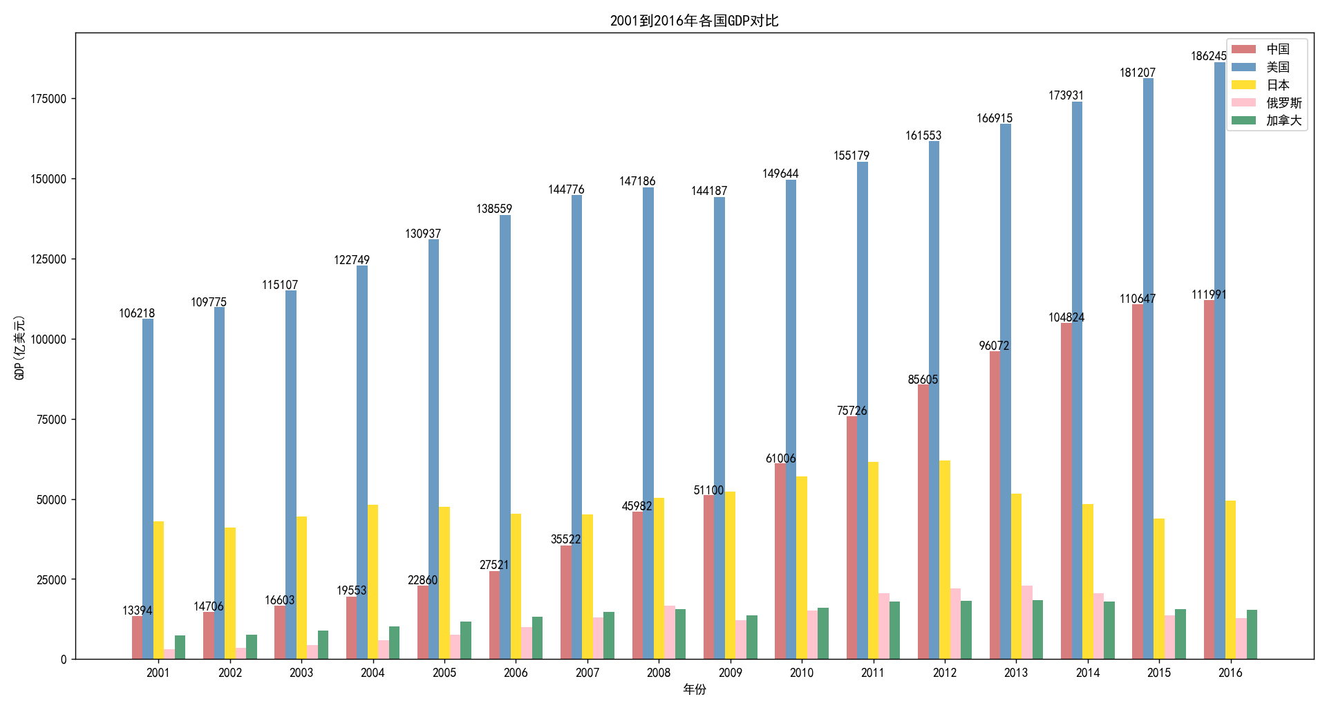
countries = ['中国', '美国', '日本', '俄罗斯', '加拿大']
# 采用循环绘制5组柱状图
for i in range(len(colors)):
# 使用自定义X坐标将数据分开
plt.bar(x=np.arange(len(x_data))+bar_width*i, height=country_gdp_list[i],
label=countries[i], color=colors[i], alpha=0.8, width=bar_width)
# 仅为中国、美国的条柱上绘制GDP数值
if i < 2:
for x, y in enumerate(country_gdp_list[i]):
plt.text(x, y + 100, '%.0f' % y, ha='center', va='bottom')
# 为X轴设置刻度值
plt.xticks(np.arange(len(x_data))+bar_width*2, x_data)
# 设置标题
plt.title("2001到2016年各国GDP对比")
# 为两条坐标轴设置名称
plt.xlabel("年份")
plt.ylabel("GDP(亿美元)")
# 显示图例
plt.legend()
plt.show()
import json
import pygal

filename = 'gdp_json.json'
# 读取JSON格式的GDP数据
with open(filename) as f:
    gpd_list = json.load(f)
pop_filename = 'population-figures-by-country.json'
# 读取JSON格式的人口数据
with open(pop_filename) as f:
    pop_list = json.load(f)

# 使用list列表依次保存美国、日本、俄罗斯、加拿大的人均GDP值
country_mean_gdps = [{}, {}, {}, {}]
country_codes = ['USA', 'JPN', 'RUS', 'CAN']
# 遍历列表的每个元素,每个元素是一个GDP数据项
for gpd_dict in gpd_list:
    for i, country_code in enumerate(country_codes):
        # 只读取指定国家的数据
        if gpd_dict['Country Code'] == country_code:
            year = gpd_dict['Year']
            # 只读取2001年到2016
            if 2017 > year > 2000:
                for pop_dict in pop_list:
                    # 获取指定国家的人口数据
                    if pop_dict['Country_Code'] == country_code:
                        # 使用该国GDP总值除以人口数量,得到人均GDP
                        country_mean_gdps[i][year] = round(gpd_dict['Value']
                            / pop_dict['Population_in_%d' % year])
# 使用list列表依次保存美国、日本、俄罗斯、加拿大的人均GDP值
country_mean_gdp_list = [[], [], [], []]
# 构建时间数据
x_data = range(2001, 2017)
for i in range(len(country_mean_gdp_list)):
    for year in x_data:
        country_mean_gdp_list[i].append(country_mean_gdps[i][year])
# 定义国家名称列表
countries = ['美国', '日本', '俄罗斯', '加拿大']
# 创建pygal.Bar对象(柱状图)
bar = pygal.Bar()
# 采用循环添加代表条柱的数据
for i in range(len(countries)):
    bar.add(countries[i], country_mean_gdp_list[i])
bar.width=1100
# 设置X轴的刻度值
bar.x_labels = x_data
bar.title = '2001到2016年各国人均GDP对比'
# 设置X、Y轴的标题
bar.x_title = '年份'
bar.y_title = '人均GDP(美元)'
# 设置X轴的刻度值旋转45度
bar.x_label_rotation = 45
# 设置将图例放在底部
bar.legend_at_bottom = True
# 指定将数据图输出到SVG文件中
bar.render_to_file('mean_gdp.svg')
数据清洗
import csv
import pygal
from datetime import datetime
from datetime import timedelta

filename = 'guangzhou-2017.csv'
# 打开文件
with open(filename) as f:
    # 创建cvs文件读取器
    reader = csv.reader(f)
    # 读取第一行,这行是表头数据。
    header_row = next(reader)
    print(header_row)

    # 准备展示的数据
    shades, sunnys, cloudys, rainys = 0, 0, 0, 0
    prev_day = datetime(2016, 12, 31)
    for row in reader:
        try:
            # 将第一列的值格式化为日期
            cur_day = datetime.strptime(row[0], '%Y-%m-%d')
            description = row[3]
        except ValueError:
            print(cur_day, '数据出现错误')
        else:
            # 计算前、后两天数据的时间差
            diff = cur_day - prev_day
            # 如果前、后两天数据的时间差不是相差一天,说明数据有问题
            if diff != timedelta(days=1):
                print('%s之前少了%d天的数据' % (cur_day, diff.days - 1))
            prev_day = cur_day
            if '阴' in description:
                shades += 1
            elif '晴' in description:
                sunnys += 1
            elif '云' in description:
                cloudys += 1
            elif '雨' in description:
                rainys += 1
            else:
                print(description)
# 创建pygal.Pie对象(饼图)
pie = pygal.Pie()
# 为饼图添加数据
pie.add("阴", shades)
pie.add("晴", sunnys)
pie.add("多云", cloudys)
pie.add("雨", rainys)
pie.title = '2017年广州天气汇总'
# 设置将图例放在底部
pie.legend_at_bottom = True
# 指定将数据图输出到SVG文件中
pie.render_to_file('guangzhou_weather.svg')
读取网络数据
import re
from datetime import datetime
from datetime import timedelta
from matplotlib import pyplot as plt
from urllib.request import *

# 定义一个函数读取lishi.tianqi.com的数据
def get_html(city, year, month):  #①
    url = 'http://lishi.tianqi.com/' + city + '/' + str(year) + str(month) + '.html'
    # 创建请求
    request = Request(url)
    # 添加请求头
    request.add_header('User-Agent', 'Mozilla/5.0 (Windows NT 10.0; WOW64)' +
        'AppleWebKit/537.36 (KHTML, like Gecko) Chrome/54.0.2840.99 Safari/537.36')
    response = urlopen(request)
    # 获取服务器响应
    return response.read().decode('gbk')

# 定义3个list列表作为展示的数据
dates, highs, lows = [], [], []
city = 'guangzhou'
year = '2017'
months = ['01', '02', '03', '04', '05', '06', '07',
    '08', '09', '10', '11', '12']
prev_day = datetime(2016, 12, 31)
# 循环读取每个月的天气数据
for month in months:
    html = get_html(city, year, month)
    # 将html响应拼起来
    text = "".join(html.split())
    # 定义包含天气信息的div的正则表达式
    patten = re.compile('<divclass="tqtongji2">(.*?)</div><divstyle="clear:both">')
    table = re.findall(patten, text)
    patten1 = re.compile('<ul>(.*?)</ul>')
    uls = re.findall(patten1, table[0])
    for ul in uls:
        # 定义解析天气信息的正则表达式
        patten2 = re.compile('<li>(.*?)</li>')
        lis = re.findall(patten2, ul)
        # 解析得到日期数据
        d_str = re.findall('>(.*?)</a>', lis[0])[0]
        try:
            # 将日期字符串格式化为日期
            cur_day = datetime.strptime(d_str, '%Y-%m-%d')
            # 解析得到最高气温和最低气温
            high = int(lis[1])
            low = int(lis[2])
        except ValueError:
            print(cur_day, '数据出现错误')
        else:
            # 计算前、后两天数据的时间差
            diff = cur_day - prev_day
            # 如果前、后两天数据的时间差不是相差一天,说明数据有问题
            if diff != timedelta(days=1):
                print('%s之前少了%d天的数据' % (cur_day, diff.days - 1))
            dates.append(cur_day)
            highs.append(high)
            lows.append(low)
            prev_day = cur_day
# 配置图形
fig = plt.figure(dpi=128, figsize=(12, 9))
# 绘制最高气温的折线
plt.plot(dates, highs, c='red', label='最高气温',
    alpha=0.5, linewidth = 2.0)
# 再绘制一条折线
plt.plot(dates, lows, c='blue', label='最低气温',
    alpha=0.5, linewidth = 2.0)
# 为两个数据的绘图区域填充颜色
plt.fill_between(dates, highs, lows, facecolor='blue', alpha=0.1)
# 设置标题
plt.title("广州%s年最高气温和最低气温" % year)
# 为两条坐标轴设置名称
plt.xlabel("日期")
# 该方法绘制斜着的日期标签
fig.autofmt_xdate()
plt.ylabel("气温(℃)")
# 显示图例
plt.legend()
ax = plt.gca()
# 设置右边坐标轴线的颜色(设置为none表示不显示)
ax.spines['right'].set_color('none')
# 设置顶部坐标轴线的颜色(设置为none表示不显示)
ax.spines['top'].set_color('none')
plt.rcParams['font.sans-serif'] = ['SimHei']
plt.rcParams['axes.unicode_minus'] = False
plt.show()


 438
438


 被折叠的 条评论
为什么被折叠?
被折叠的 条评论
为什么被折叠?
 到【灌水乐园】发言


