sklearn模型评选择与评估

最新推荐文章于 2024-06-01 21:50:07 发布

huahuahuahhhh

最新推荐文章于 2024-06-01 21:50:07 发布

阅读量790

点赞数 1

分类专栏： Sklearn_工具文章标签：模型选择与评估对数坐标系显示中文

本文链接：https://blog.csdn.net/Blankit1/article/details/105369875

版权

Sklearn_工具专栏收录该内容

4 篇文章 0 订阅

订阅专栏

在这里插入图片描述

sklearn模型评选择与评估

1. 数据集划分

在这里插入图片描述

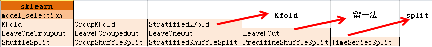
1.1 K折交叉验证

1.1.1 K折交叉验证算法原理
a. 将全部训练及S分成K个不相交的子集，假设S中样本个数为M，那么，每一个子集的训练样本个数为M/K相应的子集称做 ${S_{1},S_{2},...,S_{K}\}$
b. 每次从分好的训练只集中拿出一个测试集。其他K-1一个作为训练集。
c. 在K-1一个训练集上训练出学习器模型，把这个模型放到测试集上，得到分类率.
d. 计算K求得分类率的平均值。作为该模型的真实分类率。
在这里插入图片描述
1.1.2 StratifiedKFold划分后，训练集、测试集的比例与原始数据集一致。
1.1.3优缺点
优点：充分利用了所有样本
缺点：计算繁琐。计算K次，测试K次
1.1.4代码

返回的是每一折的索引

def KFold_practice():
    x = np.arange(12)
    X = x.reshape(6, 2)
    y = np.arange(15, 21)

    kf = model_selection.KFold(n_splits=3)  # 定义一个K折分割器  还有参数shuffle，random_state
    'KFold.split(x)返回的是索引，训练样本和测试样本是什么要将索引带到数据集中去'
    for train_index, test_index in kf.split(X):
        print("TRAIN Index:", train_index,"TEST Index:", test_index)

        X_train, X_test = X[train_index], X[test_index]
        y_train, y_test = y[train_index], y[test_index]
        print("TRAIN Subset:\n", X_train)
        print("TEST Subset:\n", X_test)
KFold_practice()

TRAIN Index: [2 3 4 5] TEST Index: [0 1]
TRAIN Subset:
 [[ 4  5]
 [ 6  7]
 [ 8  9]
 [10 11]]
TEST Subset:
 [[0 1]
 [2 3]]
TRAIN Index: [0 1 4 5] TEST Index: [2 3]
TRAIN Subset:
 [[ 0  1]
 [ 2  3]
 [ 8  9]
 [10 11]]
TEST Subset:
 [[4 5]
 [6 7]]
TRAIN Index: [0 1 2 3] TEST Index: [4 5]
TRAIN Subset:
 [[0 1]
 [2 3]
 [4 5]
 [6 7]]
TEST Subset:
 [[ 8  9]]

1.2 留一法(LOO)

1.2.1 留一法
假设在N个样本中，将每一个样本作为测试集，剩下的N-1个作为作为训练样本，这样得到N个分类器、N个测试结果，N个结果平均来衡量模型的性能。
LOO与KFold相比，当K<<N时，LOO比KFold更耗时。
1.2.2 留P法
假设在N个样本中，将P个样本作为测试集，剩下的N-P个作为作为训练样本，这样得到 $C_{n}^{P}$ 个训练-测试集对（train-test pairs），当P>1是，测试集将发生重叠。当P=1时，变成了留一法。
1.2.3 代码
与Kfold类似，划分后返回的也是索引

def leave_one_out():
    x = np.arange(5,13)
    X = x.reshape(4, 2)
    y = np.arange(15, 21)
    loo = model_selection.LeaveOneOut()
    for train_index,test_index in loo.split(X):
        print("TRAIN INDEX:", train_index, "TEST INDEX:", test_index)
        X_train, X_test = X[train_index], X[test_index]
        # y_train, y_test = y[train_index], y[test_index]
        print("TRAIN X:", X_train, "TEST X:", X_test)

1.3 随机划分法

产生指定数量的训练/测试数据集划分。指定训练集和测试集的比例或者数量。
首先对样本随机打乱，然后划分train/test对。
可以通过random_state控制随机序列发生器，使得运算结果可重现。
StratifiedShuffleSplit是ShuffleSplit的变体，返回分层划分。划分后每一个类的比例与原始数据集比例一致。

2. 超参数优化方法

2.1 网格搜索穷举式超参数优化方法

GridSearchCV(eatimator,param_grid=param_grid)
参数
eatimator:分类器
param_grid：参数网格

在这里插入图片描述

from sklearn.datasets import load_digits
from sklearn.ensemble import forest
from scipy import stats
import numpy as np
import pandas as pd

data = load_digits()
print(data.keys())
X,y = data['data'],data['target']
X_train, X_test, y_train, y_test = train_test_split(X,y,train_size=0.7,test_size=0.3)

model = forest.RandomForestClassifier(n_estimators=10)
# 待优化的超参数
print(model.get_params().keys())# 获取模型的参数名
def gridSearchCV(model):
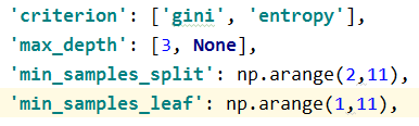
    param_grid = {
        'criterion': ['gini', 'entropy'],
        'max_depth': [3, None],
        'min_samples_split': np.arange(2,11),
        'min_samples_leaf': np.arange(1,11),
    }
    start = time.time()
    clf = GridSearchCV(model,param_grid=param_grid)
    clf.fit(X_train, y_train)
    duration = time.time() - start
    print('*best_params_*:\n', clf.best_params_)
    # print('*best_estimator_*:\n',clf.best_estimator_)
    print('模型在测试集的得分', clf.score(X_test, y_test))
    print('总共耗时：', duration)
    cv_result = pd.DataFrame.from_dict(clf.cv_results_)
    print(type(clf.cv_results_))
    print(clf.cv_results_.keys())
    # with open('GridSearchCV_result.csv', 'w') as f: cv_result.to_csv(f)

参数网格如下。一共有2*2*9*10=360种组合方式。GridSearchCV在每种参数组合下计算在N折交叉验证的每一折中计算训练集和测试集上的得分。
在这里插入图片描述
clf.cv_results_是一个字典类型的数据，结果如下。rank_test_score对应的是某中参数组合下，模型在测试集中结果的排名。

2.2 随机采样式超参数优化方法

RandomizedSearchCV(eatimator, param_distributions=param_distribution, n_iter=10,cv=3)
参数
eatimator:分类器
param_distributions：参数分布。参数值按参数分布选取
n_iter:迭代次数，选多少组参数组合
在这里插入图片描述

#模型与GridSearchCV相同
def randomizedCV(model):
    param_distribution = {

        'criterion': ['gini', 'entropy'],
        'max_depth': [3, None],
        'min_samples_split': stats.randint(2, 11),
        'min_samples_leaf': stats.randint(1, 11),
    }
    start = time.time()
    clf = RandomizedSearchCV(model, param_distributions=param_distribution, n_iter=10,cv=3)
    clf.fit(X_train, y_train)
    duration = time.time() - start
    print('*best_params_*:\n', clf.best_params_)
    # print('*best_estimator_*:\n',clf.best_estimator_)
    print(type(clf.cv_results_))
    top = 3
    # clf.cv_results_ 是选择参数的日志信息
    # cv_result = pd.DataFrame.from_dict(clf.cv_results_)
    # with open('cv_result.csv', 'w') as f: cv_result.to_csv(f)
    # report(clf.cv_results_,top)
    # # print('模型在测试集的得分', clf.score(X_test, y_test))
    # print('总共耗时：', duration)

在这里插入图片描述

3. 模型验证方法

3.1 通过交叉验证计算得分

model_selection.cross_val_score(eatimator,X,y,cv=cv,n_jobs=4)
参数
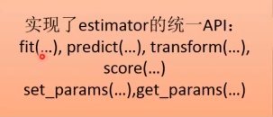
eatimator:实现fit()的学习器
X:array_like,需要学习的数据，可以是列表或2d数组
y:array_like,可选的。监督学习中样本的真实目标值
scoring:string,callable or None，可选的，默认是None
   None - 调用eatimator的score函数
   string Or callable需实现scorer(estimator,X,y)
cv: int,交叉验证生成器对象或者一个迭代器，可选的，默认None
   决定交叉验证划分策略，cv的可选项：
a. None:使用默认的3折交叉验证
b.interger：K折StratifiedKfold的K
c.交叉验证生成器对象
d.一个能产生train/test划分的迭代器对象。
返回值
scores：浮点数组，shape=len(list(cv)) 在测试集上的得分
每一次交叉验证的得分形成一个数组（默认是3折交叉验证，生成3个数组）

#coding:utf-8
from sklearn.datasets import load_digits
from sklearn.model_selection import cross_val_score,ShuffleSplit
from sklearn.svm import SVC
import numpy as np
from matplotlib import pyplot as plt
data = load_digits()
# print(data.keys())
X,y = data['data'],data['target']# data['data'] 一维数组， data['images'] 二维数组（8x8）
# print(len(X))
model = SVC(gamma=0.001)
cv = ShuffleSplit(n_splits=10,test_size=0.2)
c_s = np.logspace(-6,0,6)
print(c_s)
result = []
for c in c_s:
    model.c = c
    t = cross_val_score(model,X,y,cv=cv,n_jobs=4)
    print(np.mean(t))
    result.append(np.mean(t))
# plt.plot(c_s,result,'o')
plt.plot(c_s,result)
plt.xscale('log')# 对数坐标
plt.xlabel('c')
plt.ylabel('accuracy')
plt.rcParams['font.sans-serif']=['SimHei'] #显示中文
plt.title(r'参数c对SVM的影响')
plt.show()

在这里插入图片描述

3.2 对每个输入数据点产生交叉验证估计

model_selection .cross_val_predict(estimator,X,y=None,cv=None,n_jobs=1,method='predict')
参数

method：string,optional,default:predict. Invokes the passed method of the passed estimator.
默认使用传入模型的预测方法。

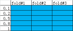
3.3 计算并绘制模型的学习率曲线

learning_curve(estimator, X, y, groups=None, train_sizes=np.linspace(0.1, 1.0, 5), cv='warn', scoring=None, exploit_incremental_learning=False, n_jobs=None, pre_dispatch="all", verbose=0, shuffle=False, random_state=None, error_score='raise-deprecating')
计算指定学习器在不同大小的训练集上经过交叉验证的训练得分和测试得分。
算法过程
首先用一个交叉验证生成器将整体数据集划分成K折，每一折划分成训练集和测试集。从每一折的训练集中取出一定比例(比如0.1)作为训练集，然后不断增加子集的比例，在这些自己上训练模型。然后计算在对应自己下的模型在整体训练集和测试集上的得分。
在这里插入图片描述
参数

train_sizes :array_like,shape(n_tricks,),dtype:float or int.
用于指定训练样本子集的相对数量或者绝对数量。
如果是浮点数，则是训练集中样本数量的百分比，(0,1]之间。
如果是整型数，则指的是训练子集的样本数量，这个数量不能超过训练样本总体数量。默认值np.linspace(0.1,1.0,5)

返回值

train_sizes_abs:array,shape=(n_unique_tricks,),dtype:int。返回train_sizes去掉重复值后的结果。
train_scores:array,shape=(n_unique_tricks,n_cv_folds),scores on training sets.
test_scores:array,shape=(n_unique_tricks,n_cv_folds),scores on testsets.

from matplotlib import pyplot as plt
import sklearn
from sklearn.datasets import load_digits
from sklearn.model_selection import learning_curve
from sklearn.model_selection import train_test_split,ShuffleSplit,RandomizedSearchCV
from sklearn.ensemble import forest

import numpy as np
data = load_digits()
print(data.keys())
X,y = data['data'],data['target']# data['data'] 一维数组， data['images'] 二维数组（8x8）
print(len(X))
# model = SVC(gamma=0.001)
model = forest.RandomForestClassifier(n_estimators=10)

cv = ShuffleSplit(n_splits=10,test_size=0.2)
clf = model
t,train_scores,test_scores = learning_curve(clf,X,y,cv=cv,n_jobs=4)
# print(t)
print('*'*20)
print('train_scores:\n',train_scores)
print('*'*20)
print('test_scores:\n',test_scores)
test_score = np.mean(test_scores,axis = 1)
print(test_score)
plt.plot(test_score)
plt.show()

在这里插入图片描述

3.4 计算并绘制模型的验证曲线

model_selection.validation_curve(estimator, X, y, param_name, param_range, groups=None, cv='warn', scoring=None, n_jobs=None, pre_dispatch="all", verbose=0, error_score='raise-deprecating')
当某个参数变化时，在该参数每一个取值下计算出模型在训练集和测试集上的得分。（与GridSearchCV类似，但是只可以计算在测试集上的得分，且只能有一个参数）
参数

param_name:string，参数名
param_range：array_like,shape(n_values,)，参数的取值范围
返回值
train_scoresarray_like,shape(n_trick,n_cv_folds),在训练集上的得分。
test_scoresarray_like,shape(n_trick,n_cv_folds),在测试集上的得分。

huahuahuahhhh

关注

1
点赞
踩
5

收藏

觉得还不错? 一键收藏
0
评论
sklearn模型评选择与评估

sklearn模型评选择与评估1. 数据集划分1.1 K折交叉验证a. 将全部训练及S分成K个不相交的子集，假设S中样本个数为M，那么，每一个子集的训练样本个数为M/K相应的子集称做{S1,S2,...,SK}\{S_{1},S_{2},...,S_{K}\}{S1,S2,...,SK}b. 每次从分好的训练只集中拿出一个测试集。其他K-1一个作为训练集。c. 在K-1一个训练...
复制链接

扫一扫