


 博客介绍了在调用kmeans函数时,其中调用的whiten函数是对输入数据按标准差做归一化处理。白化处理与标准化不同,它没有减去均值。还提到按步骤实现和调用函数实现结果相同。
调用kmeans函数,kmeans中调用了whited函数。查后,发现whiten是对输入数据按标准差做归一化处理。
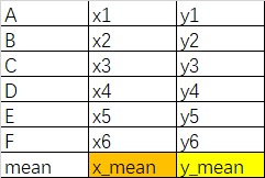
variance=Σi=1n(xi−xmean)2nvariance = \frac{ \Sigma_{i=1}^{n}(x_{i} - x_{mean})^{2}}{n}variance=nΣi=1n(xi−xmean)2
stand_devation=variancestand\_devation = \sqrt{variance}stand_devation=variance
经过whiten后
xi′=xistand_devationx_{i}^{'} =\frac{x_{i}} {stand\_devation}xi′=stand_devationxi
与标准化不同的是,白化处理没有减去均值。
下面是按步骤实现和调用函数实现,结果是一样的。
import numpy as np
from numpy import array
from scipy.cluster.vq import vq, kmeans, whiten
import matplotlib.pyplot as plt
features  = array([[ 1.9,2.3],
    [ 1.5,2.5],
    [ 0.8,0.6],
    [ 0.4,1.8],
    [ 0.1,0.1],
    [ 0.2,1.8],
    [ 2.0,0.5],
    [ 0.3,1.5],
    [ 1.0,1.0]])

mean = np.mean(features,axis=0)# 求每列的均值[0.91111111 1.34444444]
np_square = np.power(features-mean,2)#
# print('mean:\n',mean)
print('features - mean:\n',features-mean)
# print('square:\n',np_square)
mean_sqare = np.mean(np_square,axis = 0)# 方差
# print('mean_square:\n',mean_sqare)
stand_devation = np.sqrt(mean_sqare)# 标准差
# print('stand_devation:\n',stand_devation)
np_whit = features/stand_devation# scales by devation
print('******* np_white ******')
print(np_whit)

whitened = whiten(features)# 调用scipy中的函数
print('******* whitened ******')
print(whitened)
whiten后kmeans
from numpy import random
import numpy as np
from numpy import array
from scipy.cluster.vq import vq, kmeans, whiten
import matplotlib.pyplot as plt
random.seed((1000,2000))
codes = 3
kmeans(whitened,codes)
# (array([[ 2.3110306 , 2.86287398], # random
# [ 1.32544402, 0.65607529],
# [ 0.40782893, 2.02786907]]), 0.5196582527686241)
# Create 50 datapoints in two clusters a and b
pts = 50
a = np.random.multivariate_normal([0, 0], [[4, 1], [1, 4]], size=pts)# 中心点、协方差、数据量
b = np.random.multivariate_normal([30, 10],
[[10, 2], [2, 1]],
size=pts)
features = np.concatenate((a, b))
# Whiten data
whitened = whiten(features)
# Find 2 clusters in the data
codebook, distortion = kmeans(whitened, 2)# 返回聚类中心和误差
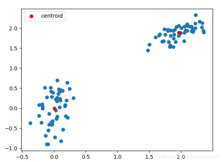
# Plot whitened data and cluster centers in red
plt.scatter(whitened[:, 0], whitened[:, 1])
# plt.scatter(features[:, 0], features[:, 1],c = 'k')
plt.scatter(codebook[:, 0], codebook[:, 1], c='r',label = 'centroid')
plt.legend()
plt.show()


 522
522

 被折叠的 条评论
为什么被折叠?
被折叠的 条评论
为什么被折叠?
 到【灌水乐园】发言


