


WRF(Weather Research and Forecasting)模型是一种广泛使用的数值天气预报模型,其输出文件通常包含大量的气象数据。使用Python可视化WRF输出文件可以提供直观的气象数据展示,有助于分析和理解模型结果。
执行wrf.exe时,如果namelist.input文件的设置的 &time_control部分 frames_per_outfile = 1000时,会将整个模拟时间输出为一个wrfout_d01*文件名,例如“wrfout_d02_2021-06-01_00%3A00%3A00”。这个文件是整个模型可视化的关键文件,接下来笔者所用的都是这个文件来进行绘制,读者根据自己的电脑设置来执行相应的代码。
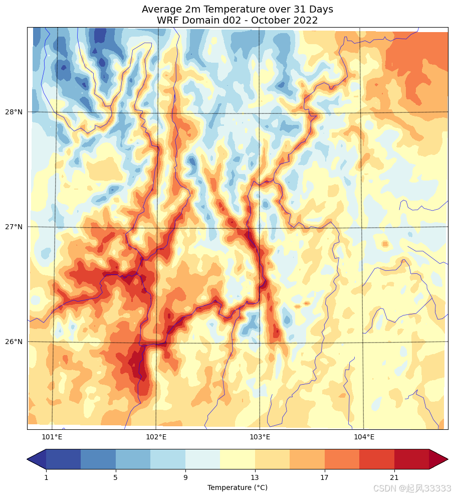
下图是绘制温度图的效果
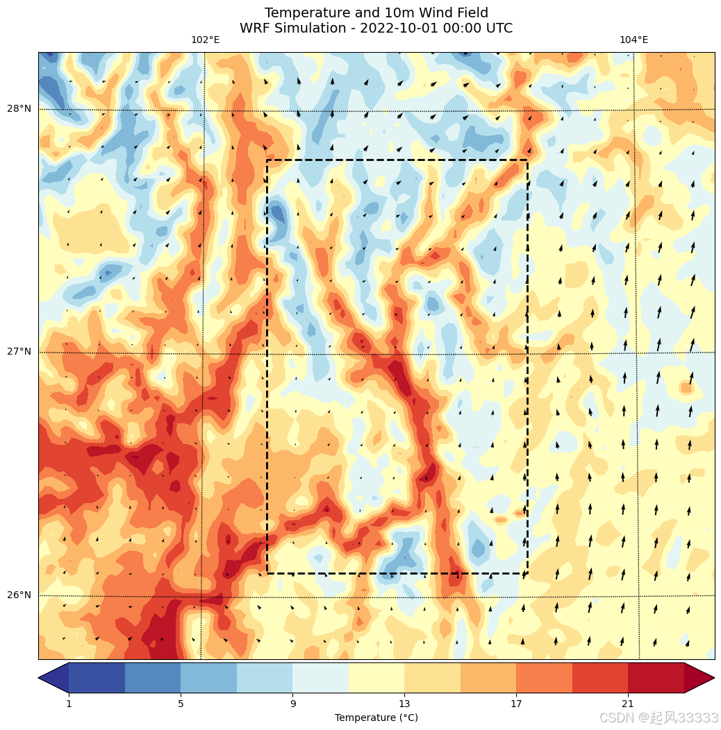
下是温度风场图的效果图(添加数据框)
1 python环境配置
因为是使用python来进行可视化,如果读者没有在本机电脑上配置过相应的python环境的可以参考下几篇文章进行python环境配置python3.9。如果是新手推荐使用conda或anaconda来配置python环境,参考第二或者第三篇文章。
注意:这里使用Basemap包来进行创建地图投影和底图的要素绘制,Basemap官方已于2020年停止维护basemap包,所以需要配置python3.9及以下版本才能下载和使用Basemap包。
Python环境配置保姆级教程(20W+阅读)
安装conda搭建python环境(保姆级教程)
目前python已经更新到3.13版本,所以笔者推荐配置一个python 3.12和一个python 3.9版本,因为3.12版本区域稳定,能够满足绝大多数使用python场景。
python官方网址:Welcome to Python.org
2 绘制温度图
下面就开始介绍使用python绘制温度图。
note:笔者使用的环境是python 3.9.19,使用的软件是visual studio Code 2020,jupyternotebook运行代码。关于jupyter notebook介绍和安装见文章:VsCode 安装Jupyter Notebook。
2.1 安装所需要的包
下指令是一尺执行,
# 基础科学计算库
pip install numpy
# NetCDF文件处理
pip install netCDF4
# 数据可视化核心库
pip install matplotlib
推荐使用conda安装basemap,如果出现下载失败的情况,可以尝试科学上网重新执行。
# 地理绘图扩展库 (需先安装依赖)
conda install -c conda-forge basemap basemap官方文档:basemap 1.4.1 documentation - Matplotlib
2.2 绘制温度图
导入相应的包
import numpy as np

import netCDF4 as nc

import matplotlib.pyplot as plt

from mpl_toolkits.basemap import Basemap

import matplotlib.cm as cm

from datetime import datetime
# 文件路径设置,将r' ' 单引号里面的内容替换为自己wrfout文件的路径。
wrf_file = r'F:\WRF\out\\wrfout_d02_2022-10-01_00%3A00%3A00'下面的解释都在代码里用" # "注释了。
# 读取WRF数据
    ds = nc.Dataset(wrf_file)

    # 获取地理坐标
    lon = ds.variables['XLONG'][0]  # 经度(2D)
    lat = ds.variables['XLAT'][0]   # 纬度(2D)

    # 时间处理(示例取第一个时间步)
    time_idx = 0
    time_str = ''.join([x.decode('utf-8') for x in ds.variables['Times'][time_idx]])
    plot_time = datetime.strptime(time_str, '%Y-%m-%d_%H:%M:%S')

    # 提取并转换温度数据(K → ℃)
    if 'T2' in ds.variables:
        temp_k = ds.variables['T2'][:, :, :]  # 所有时次的2米气温
        temp_c = temp_k - 273.15
        mean_temp_c = np.mean(temp_c, axis=0)  # 计算平均温度
    else:
        raise ValueError("T2 variable not found in the dataset")


    # 创建地图投影
    plt.figure(figsize=(16, 12))
    m = Basemap(projection='lcc',
            llcrnrlon=lon.min() + 0.5, urcrnrlon=lon.max() - 0.5,
            llcrnrlat=lat.min() + 0.5, urcrnrlat=lat.max() - 0.5,
            lat_0=lat.mean(), lon_0=lon.mean(),
            resolution='i', area_thresh=1000)

    # 转换坐标到投影空间
    x, y = m(lon, lat)

    # 绘制基础地理要素
    m.drawcoastlines(linewidth=0.8)
    m.drawcountries(linewidth=0.5)
    m.drawstates(linestyle=':')
    parallels = np.arange(int(lat.min()), int(lat.max())+1, 1)
    meridians = np.arange(int(lon.min()), int(lon.max())+1, 2)  # 每隔2度显示一个经度标签
    m.drawparallels(parallels, labels=[1,0,0,0], fontsize=10)  # 纬度标签显示在左侧
    m.drawmeridians(meridians, labels=[0,0,1,1], fontsize=10)  # 经度标签显示在底部和右侧


    # 绘制温度填色图
    levels_temp = np.arange(np.floor(mean_temp_c.min()), np.ceil(mean_temp_c.max()) + 1, 2)
    cs_temp = m.contourf(x, y, mean_temp_c, levels=levels_temp, cmap='RdYlBu_r', extend='both')
    cbar_temp = m.colorbar(cs_temp, location='bottom', pad=0.05, label='Temperature (°C)')


    # 添加矢量图例
    plt.quiverkey(q, 0.85, 0.1, 10, '10 m/s', coordinates='figure')


    # 添加标题
    plt.title(f'Temperature and 10m Wind Field\nWRF Simulation - {plot_time.strftime("%Y-%m-%d %H:%M UTC")}',
              fontsize=14, pad=20)

    # 保存输出
    plt.savefig('temp_wind_field.png', dpi=300, bbox_inches='tight')
    plt.show()
可以添加数据框,由读者自己选择
# 定义数据框范围中的四个变量由读者自己定义。
rect_lon_min, rect_lon_max = 经度左范围, 经度右范围 左右
rect_lat_min, rect_lat_max = 纬度上范围, 纬度下范围 上下
    # 定义数据框范围
    rect_lon_min, rect_lon_max = 102.3, 103.5
    rect_lat_min, rect_lat_max = 26.1, 27.8

    # 将数据框范围转换为投影坐标
    rect_x_min, rect_y_min = m(rect_lon_min, rect_lat_min)
    rect_x_max, rect_y_max = m(rect_lon_max, rect_lat_max)

    # 绘制数据框
    m.plot([rect_x_min, rect_x_max, rect_x_max, rect_x_min, rect_x_min],
           [rect_y_min, rect_y_min, rect_y_max, rect_y_max, rect_y_min],
           color='black', linewidth=2,linestyle='--')
风场图的代码
# 提取10米风速分量(注意维度顺序)
    u10 = ds.variables['U10'][time_idx]  # 东向分量
    v10 = ds.variables['V10'][time_idx]  # 北向分量

    # 计算风速大小和风向
    wind_speed = np.sqrt(u10**2 + v10**2)  # 风速(m/s)
    wind_dir = np.arctan2(-u10, -v10) * (180 / np.pi)  # 风向(度)
    wind_dir = (wind_dir + 360) % 360  # 转换为0-360度

    # 绘制风速矢量箭头(每隔5个点采样)
    step = 5
    q = m.quiver(x[::step, ::step], y[::step, ::step],
                 u10[::step, ::step], v10[::step, ::step],
                 scale=200, width=0.002, headwidth=3)  # 减小scale以使箭头更长
3 完整代码展示
3.1 温度图代码
import numpy as np
import netCDF4 as nc
import matplotlib.pyplot as plt
from mpl_toolkits.basemap import Basemap
import os

# 解决路径转义问题(Windows系统需要)
file_path = r'F:\WRF\out\2022.10.1-31\wrfout_d02_2022-10-01_00%3A00%3A00'

try:
    # 读取WRF输出文件
    dataset = nc.Dataset(file_path)

    # 提取地理坐标(注意WRF的坐标变量名)
    lons = dataset.variables['XLONG'][0, :, :]  # 经度(二维数组)
    lats = dataset.variables['XLAT'][0, :, :]   # 纬度(二维数组)

    # 提取并转换温度数据(K → ℃)
    if 'T2' in dataset.variables:
        temp_k = dataset.variables['T2'][:, :, :]  # 所有时次的2米气温
        temp_c = temp_k - 273.15
        mean_temp_c = np.mean(temp_c, axis=0)  # 计算平均温度
    else:
        raise ValueError("T2 variable not found in the dataset")

    # 创建地图投影(推荐使用Lambert投影,需根据实际域设置参数)
    plt.figure(figsize=(14, 10))
    map_proj = Basemap(projection='lcc',
                       llcrnrlon=lons.min(), urcrnrlon=lons.max(),
                       llcrnrlat=lats.min(), urcrnrlat=lats.max(),
                       lat_0=np.mean(lats), lon_0=np.mean(lons),
                       resolution='i', area_thresh=1000)

    # 转换坐标到投影空间
    x, y = map_proj(lons, lats)

    # 绘制基础地理要素
    map_proj.drawcoastlines(linewidth=0.5)
    map_proj.drawcountries(linewidth=0.5)
    map_proj.drawstates()  # 添加州/省界
    map_proj.drawrivers(color='blue')  # 添加河流

    # 创建颜色分级(示例:每2℃一个色阶)
    levels = np.arange(np.floor(mean_temp_c.min()), np.ceil(mean_temp_c.max()) + 1, 2)

    # 绘制填色图
    cs = map_proj.contourf(x, y, mean_temp_c, levels=levels, cmap='RdYlBu_r', extend='both')

    # 添加颜色条
    cbar = map_proj.colorbar(cs, location='bottom', pad="5%", label='Temperature (°C)')

    # 添加标题和网格
    plt.title('Average 2m Temperature over 31 Days\nWRF Domain d02 - October 2022', fontsize=14)
    map_proj.drawparallels(np.arange(-90, 90, 1), labels=[1,0,0,0], fontsize=10)
    map_proj.drawmeridians(np.arange(-180, 180, 1), labels=[0,0,0,1], fontsize=10)

    # 显示图形
    plt.tight_layout()
    plt.show()

except Exception as e:
    print(f"Error occurred: {str(e)}")
finally:
    if 'dataset' in locals():
        dataset.close()
3.2 温度风场图代码(添加数据框)
如果需要单独的风场图参考博客:WRF输出结果的可视化展示与分析:以风速为例
import numpy as np
import netCDF4 as nc
import matplotlib.pyplot as plt
from mpl_toolkits.basemap import Basemap
import matplotlib.cm as cm
from datetime import datetime

# 文件路径设置
wrf_file = r'F:\WRF\out\2022.10.1-31\wrfout_d02_2022-10-01_00%3A00%3A00'

try:
    # 读取WRF数据
    ds = nc.Dataset(wrf_file)

    # 获取地理坐标
    lon = ds.variables['XLONG'][0]  # 经度(2D)
    lat = ds.variables['XLAT'][0]   # 纬度(2D)

    # 时间处理(示例取第一个时间步)
    time_idx = 0
    time_str = ''.join([x.decode('utf-8') for x in ds.variables['Times'][time_idx]])
    plot_time = datetime.strptime(time_str, '%Y-%m-%d_%H:%M:%S')

    # 提取并转换温度数据(K → ℃)
    if 'T2' in ds.variables:
        temp_k = ds.variables['T2'][:, :, :]  # 所有时次的2米气温
        temp_c = temp_k - 273.15
        mean_temp_c = np.mean(temp_c, axis=0)  # 计算平均温度
    else:
        raise ValueError("T2 variable not found in the dataset")

    # 提取10米风速分量(注意维度顺序)
    u10 = ds.variables['U10'][time_idx]  # 东向分量
    v10 = ds.variables['V10'][time_idx]  # 北向分量

    # 计算风速大小和风向
    wind_speed = np.sqrt(u10**2 + v10**2)  # 风速(m/s)
    wind_dir = np.arctan2(-u10, -v10) * (180 / np.pi)  # 风向(度)
    wind_dir = (wind_dir + 360) % 360  # 转换为0-360度

    # 创建地图投影
    plt.figure(figsize=(16, 12))
    m = Basemap(projection='lcc',
            llcrnrlon=lon.min() + 0.5, urcrnrlon=lon.max() - 0.5,
            llcrnrlat=lat.min() + 0.5, urcrnrlat=lat.max() - 0.5,
            lat_0=lat.mean(), lon_0=lon.mean(),
            resolution='i', area_thresh=1000)

    # 转换坐标到投影空间
    x, y = m(lon, lat)

    # 绘制基础地理要素
    m.drawcoastlines(linewidth=0.8)
    m.drawcountries(linewidth=0.5)
    m.drawstates(linestyle=':')
    parallels = np.arange(int(lat.min()), int(lat.max())+1, 1)
    meridians = np.arange(int(lon.min()), int(lon.max())+1, 2)  # 每隔2度显示一个经度标签
    m.drawparallels(parallels, labels=[1,0,0,0], fontsize=10)  # 纬度标签显示在左侧
    m.drawmeridians(meridians, labels=[0,0,1,1], fontsize=10)  # 经度标签显示在底部和右侧


    # 绘制温度填色图
    levels_temp = np.arange(np.floor(mean_temp_c.min()), np.ceil(mean_temp_c.max()) + 1, 2)
    cs_temp = m.contourf(x, y, mean_temp_c, levels=levels_temp, cmap='RdYlBu_r', extend='both')
    cbar_temp = m.colorbar(cs_temp, location='bottom', pad=0.05, label='Temperature (°C)')

    # 绘制风速矢量箭头(每隔5个点采样)
    step = 5
    q = m.quiver(x[::step, ::step], y[::step, ::step],
                 u10[::step, ::step], v10[::step, ::step],
                 scale=200, width=0.002, headwidth=3)  # 减小scale以使箭头更长

    # 添加矢量图例
    plt.quiverkey(q, 0.85, 0.1, 10, '10 m/s', coordinates='figure')

    # 定义数据框范围
    rect_lon_min, rect_lon_max = 102.3, 103.5
    rect_lat_min, rect_lat_max = 26.1, 27.8

    # 将数据框范围转换为投影坐标
    rect_x_min, rect_y_min = m(rect_lon_min, rect_lat_min)
    rect_x_max, rect_y_max = m(rect_lon_max, rect_lat_max)

    # 绘制数据框
    m.plot([rect_x_min, rect_x_max, rect_x_max, rect_x_min, rect_x_min],
           [rect_y_min, rect_y_min, rect_y_max, rect_y_max, rect_y_min],
           color='black', linewidth=2,linestyle='--')

    # 添加标题
    plt.title(f'Temperature and 10m Wind Field\nWRF Simulation - {plot_time.strftime("%Y-%m-%d %H:%M UTC")}',
              fontsize=14, pad=20)

    # 保存输出
    plt.savefig('temp_wind_field.png', dpi=300, bbox_inches='tight')
    plt.show()

except Exception as e:
    print(f"Error: {str(e)}")
finally:
    if 'ds' in locals():
        ds.close()
note:上面的所有代码都是按照笔者的个人喜好设计,读者按需更改颜色色带和风场箭头大小等。


 3620
3620

 被折叠的 条评论
为什么被折叠?
被折叠的 条评论
为什么被折叠?
 到【灌水乐园】发言


