自适应控制——RELS、MVC(参数已知)、MVSTC(参数未知)

1.递推增广最小二乘估计(RELS)
仿真系统：
y(k)-1.5y(k-1)+0.7y(k-2)=u(k-3)+0.5u(k-4)+e(k)-e(k-1)+0.2e(k-2);
e(k)为k时刻的白噪声值

%递推增广最小二乘法
clear
clc

L = 1000;
a=[-1.5 0.7];b=[1,0.5];c=[1,-1,0.2];%系统输入输出表达式
e = 0.1*randn(L,1);e0 = zeros(1,2);%精确干扰 用于求精确输出 e(i-1) e(i-2)
e_hat = zeros(1,2);%干扰的估计值 e_hat(i-1) e_hat(i-2)
y = zeros(L,1);y0 = zeros(1,2);%y(i-1) y(i-2)
u = randn(L,1);u0 = zeros(1,4);%u(i-1) u(i-2) u(i-3) u(i-4)
seeta = zeros(6,L);seeta_stand = [a,b,c(2:3)];seeta0=zeros(6,1);
P = 10^6*eye(6);
fa = zeros(1,6);
for i = 1:L
    fa = [-y0,u0(3:4),e0]';
    y(i) = fa'*seeta_stand' + e(i);
    
    fa_hat = [-y0,u0(3:4),e_hat]';
    K = P*fa_hat/(1+fa_hat'*P*fa_hat);
    seeta(:,i) = seeta0 + K*[y(i)-fa_hat'*seeta0];
    P=[eye(6)-K*fa_hat']*P;
    
    ee = y(i) - fa_hat'*seeta(:,i);%误差最前值
    seeta0 = seeta(:,i);
    for ie = length(e0):-1:2
        e0(ie) = e0(ie-1);
    end
    e0(1) = e(i);
    for ie_hat = length(e_hat):-1:2
        e_hat(ie_hat) = e_hat(ie_hat-1);
    end
    e_hat(1) = ee;
    for iu = length(u0):-1:2
        u0(iu) = u0(iu-1);
    end
    u0(1) = u(i);
    for iy = length(y0):-1:2
        y0(iy) = y0(iy-1);
    end
    y0(1) = y(i);
end
x = 1:L
subplot(3,1,1);plot(x,seeta(1,:),x,seeta(2,:));legend('a0','a1');title('a的辨识结果');
subplot(3,1,2);plot(x,seeta(3,:),x,seeta(4,:));legend('b0','b1');title('b的辨识结果');
subplot(3,1,3);plot(x,seeta(5,:),x,seeta(6,:));legend('c0','c1');title('c的辨识结果');


    

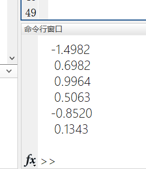
参数估计结果：


2.最小方差控制(MVC)
仿真系统：
y(k)-1.7y(k-1)+0.7y(k-2)=u(k-4)+0.5u(k-5)+e(k)+0.2e(k-2);
e(k)为k时刻的白噪声值
理想输出为一个正弦信号

%最小方差控制  P105 仿真实例4.3
clear
clc
a=[1 -1.7 0.7];b=[1 0.5];c=[1 0.2];d=4;
na = length(a);nb = length(b);nc = length(c);
L=1000;
noise = 0.1*randn(L+10,1);noise0 = [noise(1) 0];%噪音noise(i) noise(i-1)  
u = zeros(L,1);u0 = zeros(1,5);%输入 u(i-1) u(i-2) u(i-3) u(i-4) u(i-5) 
y =zeros(L,1);y0 = zeros(1,2);%输出y(i) y(i-1) y(i-2)
%yr = 10*[ones(1,L/4) -1*ones(1,L/4) ones(1,L/4) -1*ones(1,L/4)];
for i = 1:L
    yr(i) = sin((pi)/100*i);
end
yr0 = [yr(5) yr(4)];
[e,f,g] = sindiophantine(a,b,c,d);
for i = 1:L
    y(i) = -a(2:3)*y0' + b*u0(4:5)' + c*noise0';
    for iy = 2:-1:2
        y0(iy) = y0(iy - 1);
    end
    y0(1) = y(i);
    u(i) = -f(2:5)*u0(1:4)' + c*yr0' - g*y0';
    for iyr = 2:2
        yr0(iyr) = yr0(iyr-1);
    end
    num_iyr = i+5;
    if i+5>L
        num_iyr = L;
    end
    yr0(1) = yr(num_iyr);
    
    for iu = 5:-1:2
        u0(iu) = u0(iu-1);
    end
    u0(1) = u(i);
    for in = 2:2
        noise0(in) = noise0(in-1);
    end
    noise0(1) = noise(i+1);
end
x = 1:L;
plot(x,yr,'--',x,y);axis([0 1000 -10 10]);

系统输出跟随结果：

3.最小方差间接自校正控制(MVSTC)
仿真系统：
y(k)-1.7y(k-1)+0.7y(k-2)=u(k-4)+0.5u(k-5)+e(k)+0.2e(k-1);
e(k)为k时刻的白噪声值
理想输出为一个幅值为10的方波信号

%最小方差间接自校正控制  P108
%递推增广最小二乘法
clear
clc
%参数估计部分
L = 800;
a=[-1.7 0.7];b=[1,0.5];c=[1,0.2];%系统输入输出表达式
e = 0.1*randn(L,1);e0 = zeros(1,1);%精确干扰 用于求精确输出 e(i-1) 
e_hat = 0;%干扰的估计值 e_hat(i-1) 
y = zeros(L,1);y0 = zeros(1,2);%y(i-1) y(i-2)
u = zeros(L,1);u0 = zeros(1,5);%u(i-1) u(i-2) u(i-3) u(i-4) u(i-5)
seeta = zeros(5,L);seeta_stand = [a,b,c(2)];seeta0=0.001*ones(5,1);
P = 10^6*eye(5);
fa = zeros(1,5);

%自校正部分
yr = 10*[ones(1,L/4),-ones(1,L/4),ones(1,L/4),-ones(1,L/4)];%理想输出
yr0 = [yr(5) yr(4)];
%a_hat = [1 seeta0(1:2)];b_hat = [seeta0(3:4)];c_hat=[seeta0(5)];
for i = 1:L
    fa = [-y0,u0(4:5),e0]';
    y(i) = fa'*seeta_stand' + e(i);
    
    fa_hat = [-y0,u0(4:5),e_hat]';
    K = P*fa_hat/(1+fa_hat'*P*fa_hat);
    seeta(:,i) = seeta0 + K*[y(i)-fa_hat'*seeta0];
    P=[eye(5)-K*fa_hat']*P;
    
    ee = y(i) - fa_hat'*seeta(:,i);%误差最前值
    %开始自校正
    for iy = length(y0):-1:2
        y0(iy) = y0(iy-1);
    end
    y0(1) = y(i);%更新y至y(i) y(i-1)
    
    a_hat = [1 seeta0(1) seeta0(2)];b_hat = [seeta0(3) seeta0(4)];c_hat=[seeta0(5)];d=4;
    [e1,f1,g1] = sindiophantine(a_hat,b_hat,c_hat,d);
    nf1 = 5;%1 z-1 z-2 z-3
    u(i) = -(f1(2:nf1)*u0(1:4)') + c*yr0' - g1*y0';
    for iyr = 2:2
        yr0(iyr) = yr0(iyr-1);
    end
    num_iyr = i+5;
    if i+5>L
        num_iyr = L;
    end
    yr0(1) = yr(num_iyr);
    
    seeta0 = seeta(:,i);
    e0 = e(i);
    for ie_hat = length(e_hat):-1:2
        e_hat(ie_hat) = e_hat(ie_hat-1);
    end
    e_hat(1) = ee;
    for iu = length(u0):-1:2
        u0(iu) = u0(iu-1);
    end
    u0(1) = u(i);
    
end
x = 1:L;
subplot(2,2,1);plot(x,seeta(1,:),x,seeta(2,:));legend('a0','a1');title('a的辨识结果');
subplot(2,2,2);plot(x,seeta(3,:),x,seeta(4,:));legend('b0','b1');title('b的辨识结果');
subplot(2,2,3);plot(x,seeta(5,:));legend('c0','c1');title('c的辨识结果');
subplot(2,2,4);plot(x,y,'--',x,yr);legend('实际输出','理想输出');title('输出跟随情况');axis([0 L -20 20]);
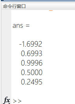
seeta(:,L)


    

仿真结果：

最后一次的估计参数