


文章目录
前言
见《开箱报告,Simulink Toolbox库模块使用指南(一)——powergui模块》
见《开箱报告,Simulink Toolbox库模块使用指南(二)——MATLAB Fuction模块》
见《开箱报告,Simulink Toolbox库模块使用指南(三)——Simscape 电路仿真模块》
见《开箱报告,Simulink Toolbox库模块使用指南(四)——S-Fuction模块》
C MEX S-Function
C MEX S-Function是使用C语言开发的一种S-Fuction,具备前一篇文章中讲解的S-Fuction的全部基本特性。它对应S-Fuction中的Level2类型,支持访问更广泛的 S-Function API 集,并支持代码生成。由于汽车电子工程与C语言密不可分,所以我们必须对C MEX S-Function重点关注。
Mathworks官方Help对该模块的说明如下所示。

本文以DFT算法为例,介绍如何利用C MEX S-Function搭建项目需求中高度自定义的信号解耦模块。
算法原理
傅里叶变换告诉我们,任何周期信号都可以分解为正弦波的叠加。具体的做法是:将被求解的原始信号,与目标频率的信号相乘,然后再积分,就得到了原始信号在该频率上的分量,公式如下:
原始信号:S;
目标频率信号:D_cos = cos(2pi*w*t);
目标频率信号:D_sin = sin(2pi*w*t);
目标信号实部:D_real = dot(S,D_cos)/N*2;
目标信号虚部:D_imag = dot(S,D_sin)/N*2;
目标信号模数:D_modl = sqrt(D_real^2 + D_imag^2);
原始信号创建
这里沿用前一篇文章中的电路方程模型,见《开箱报告,Simulink Toolbox库模块使用指南(四)——S-Fuction模块》
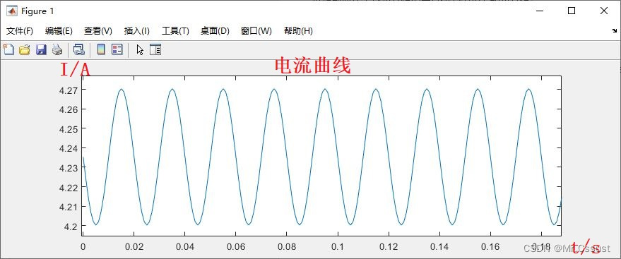
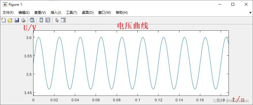
创建电压和电流信号如下:
t(S) = (0 : 4999)*0.0001;
I(A) = 4.235 + 0.035*sin(2pi * 50t + pi);
U(A) = 3.529 + 0.071*sin(2pi * 50t);
在Matlab的命令窗口中运行该动态方程,得到的电流和电压曲线,与前一篇文章一致,如下所示:
编写S函数
根据官方的Basic C MEX S-Function模板,写出的S函数完整代码如下:
#define S_FUNCTION_NAME  DFT_CMexSfunc    //函数名字,与C文件名一致
#define S_FUNCTION_LEVEL 2
#include "simstruc.h"    //Matlab宏函数库

static real_T Fs = 10e3;    //信号采样频率,与信号源一致
static real_T L = 5e3;      //信号采样点个数,两者根据Nyquist定理计算

/* Function: mdlInitializeSizes ===============================================
 * Abstract:
 *    The sizes information is used by Simulink to determine the S-function
 *    block's characteristics (number of inputs, outputs, states, etc.).
 */
static void mdlInitializeSizes(SimStruct *S)
{
	//一个算法参数Freq,目标解算频率
    ssSetNumSFcnParams(S, 1);  /* Number of expected parameters */
    if (ssGetNumSFcnParams(S) != ssGetSFcnParamsCount(S)) {
        /* Return if number of expected != number of actual parameters */
        return;
    }

    ssSetNumContStates(S, 0);
    ssSetNumDiscStates(S, 4);      //离散状态的个数

    if (!ssSetNumInputPorts(S, 1)) return;
    ssSetInputPortWidth(S, 0, 1);      //一个信号输入端口,信号维度1
    ssSetInputPortRequiredContiguous(S, 0, true); /*direct input signal access*/
    /*
     * Set direct feedthrough flag (1=yes, 0=no).
     * A port has direct feedthrough if the input is used in either
     * the mdlOutputs or mdlGetTimeOfNextVarHit functions.
     */
    ssSetInputPortDirectFeedThrough(S, 0, 1);

    if (!ssSetNumOutputPorts(S, 1)) return;
    ssSetOutputPortWidth(S, 0, 1);      //一个信号输出端口,信号维度1

    ssSetNumSampleTimes(S, 1);
    ssSetNumRWork(S, 0);
    ssSetNumIWork(S, 0);
    ssSetNumPWork(S, 0);
    ssSetNumModes(S, 0);
    ssSetNumNonsampledZCs(S, 0);

    /* Specify the operating point save/restore compliance to be same as a
     * built-in block */
    ssSetOperatingPointCompliance(S, USE_DEFAULT_OPERATING_POINT);

    ssSetOptions(S, 0);
}

/* Function: mdlInitializeSampleTimes =========================================
 * Abstract:
 *    This function is used to specify the sample time(s) for your
 *    S-function. You must register the same number of sample times as
 *    specified in ssSetNumSampleTimes.
 */
static void mdlInitializeSampleTimes(SimStruct *S)
{
//     ssSetSampleTime(S, 0, CONTINUOUS_SAMPLE_TIME);
    ssSetSampleTime(S, 0, 0.001);     //算法运行周期0.001s,不同于信号采样频率
    ssSetOffsetTime(S, 0, 0.0);

}

#define MDL_INITIALIZE_CONDITIONS   /* Change to #undef to remove function */
#if defined(MDL_INITIALIZE_CONDITIONS)
  /* Function: mdlInitializeConditions ========================================
   * Abstract:
   *    In this function, you should initialize the continuous and discrete
   *    states for your S-function block.  The initial states are placed
   *    in the state vector, ssGetContStates(S) or ssGetRealDiscStates(S).
   *    You can also perform any other initialization activities that your
   *    S-function may require. Note, this routine will be called at the
   *    start of simulation and if it is present in an enabled subsystem
   *    configured to reset states, it will be call when the enabled subsystem
   *    restarts execution to reset the states.
   */
  static void mdlInitializeConditions(SimStruct *S)
  {
     //离散状态赋初值
      real_T Count = 1;
      real_T t = 0;
      real_T cos_integ = 0;
      real_T sin_integ = 0;

      real_T *x0 = ssGetRealDiscStates(S);
      *x0++ = Count;
      *x0++ = t;
      *x0++ = cos_integ;
      *x0++ = sin_integ;
  }
#endif /* MDL_INITIALIZE_CONDITIONS */

#define MDL_START  /* Change to #undef to remove function */
#if defined(MDL_START)
  /* Function: mdlStart =======================================================
   * Abstract:
   *    This function is called once at start of model execution. If you
   *    have states that should be initialized once, this is the place
   *    to do it.
   */
  static void mdlStart(SimStruct *S)
  {
  }
#endif /*  MDL_START */

/* Function: mdlOutputs =======================================================
 * Abstract:
 *    In this function, you compute the outputs of your S-function
 *    block.
 */
static void mdlOutputs(SimStruct *S, int_T tid)
{
      real_T real = 0;
      real_T imag = 0;
      real_T modl = 0;
      real_T *y = ssGetOutputPortSignal(S,0);
      real_T *x = ssGetRealDiscStates(S);
    if(x[0]==L+1)
    {
        real = x[2]/L*2;
        imag = x[3]/L*2;
        modl = sqrt(real*real + imag*imag);
        y[0] = modl;       //解算结果输出
    }
}

#define MDL_UPDATE  /* Change to #undef to remove function */
#if defined(MDL_UPDATE)
  /* Function: mdlUpdate ======================================================
   * Abstract:
   *    This function is called once for every major integration time step.
   *    Discrete states are typically updated here, but this function is useful
   *    for performing any tasks that should only take place once per
   *    integration step.
   */
  static void mdlUpdate(SimStruct *S, int_T tid)
  {
      real_T Sr_cos;
      real_T Sr_sin;
      real_T T;
      real_T Freq = (real_T) *mxGetPr(ssGetSFcnParam(S,0));
      real_T *x = ssGetRealDiscStates(S);
      const real_T *u = (const real_T*) ssGetInputPortSignal(S,0);

      if(x[0]<=L)
      {
          Sr_cos = cos(2*3.14 * Freq*x[1]);
          Sr_sin = sin(2*3.14 * Freq*x[1]);
          x[2] = x[2] + u[0]*Sr_cos;
          x[3] = x[3] + u[0]*Sr_sin;

          x[0] = x[0] + 1;
          T = 1/Fs;
          x[1] = x[1] + T;
      }
  }
#endif /* MDL_UPDATE */

/* Function: mdlTerminate =====================================================
 * Abstract:
 *    In this function, you should perform any actions that are necessary
 *    at the termination of a simulation.  For example, if memory was
 *    allocated in mdlStart, this is the place to free it.
 */
static void mdlTerminate(SimStruct *S)
{
}
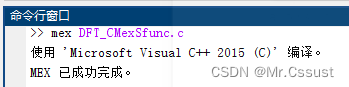
C代码编写好之后,用Matlab指令 'mex DFT_CMexSfunc.c' 进行编译。如果代码没有错误,编译成功后会看到如下提示:
仿真验证
将上述编写好的C MEX S-Fuction模块,放入Simulink模型中进行验证,如下所示:
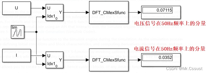
运行上述模型,得到的电流和电压如上图所示,也与前一篇文章一致。
至此,可以证明该C MEX S-Fuction模块可以较好地求解,耦合信号中的自信号分量。
Tips
C MEX S-Fuction模块能够让使用者充分自由地开发Simulink模块,一方面是跨语言的程序开发方式,只需要include其他c文件的头文件,即可调用其中已开发和验证好的c函数。另一方面是大量的能够与Simulink引擎交互的的宏函数,使得开发人员有了更大的发挥空间。一些常用的,必须熟练掌握宏函数如下:
1.系统输入宏函数
ssSetNumInputPorts(S, 1)
ssSetInputPortWidth(S, 0, 1)
ssSetInputPortDirectFeedThrough(S, 0, 1)
real_T *u = (real_T*) ssGetInputPortSignal(S,0);
Temp = u[0];
2.系统参数宏函数
ssSetNumSFcnParams(S, 1);
real_T Pa1 = (real_T) *mxGetPr(ssGetSFcnParam(S,0));
//real_T Pa2 = (real_T) *mxGetPr(ssGetSFcnParam(S,1));
Temp = Pa1;
3.系统周期宏函数
ssSetSampleTime(S, 0, 0.001);
ssSetOffsetTime(S, 0, 0.0);
4.系统状态宏函数
ssSetNumDiscStates(S, 4);
real_T *x = ssGetRealDiscStates(S);
*x++ = a;
*x++ = b;
*x++ = c;
*x++ = d;
x[0] = x[0] + 1;
x[1] = x[1] + 1;
x[2] = x[2] + 1;
x[3] = x[3] + 1;
5.系统输出宏函数
ssSetNumOutputPorts(S, 1)
ssSetOutputPortWidth(S, 0, 1)
real_T *y = ssGetOutputPortSignal(S,0);
y[0] = a;
//y[1] = b;
//y[2] = c;
//y[3] = d;
分析和应用
C MEX S-Fuction是S-Fuction的一种,他们的相同点一样,不同点在于灵活度和自由度进一步延伸,功能进一步扩展。比如本文举例的DFT求解模块,是在原有DFT算法的基础上进一步裁剪,只求解目标期望频率上的信号分量,并且把原本算法中集中计算的几个向量积分、乘除、开方等运算分解到每一个运算周期中,变成单个变量的运算(需要时还可以灵活调整指定N个周期把算法执行完),以此通过延长运算时间来节省算法对单个周期硬件算力的开销,不仅能够保证整个系统的实时性能,还能大大提高算法求解得数据量,以此提高求解精度。同时本文举例的DFT求解求解算法也是以前开发的,经过验证的模块功能,利用C MEX S-Fuction提供的C函数调用机制,无缝衔接的移植了过来。
总结
以上就是本人在使用C MEX S-Fuction模块时,一些个人理解和分析的总结,首先介绍了该模块的背景知识,然后展示它的使用方法,最后分析了该模块的特点和适用场景。
后续还会分享另外几个最近总结的Simulink Toolbox库模块,欢迎评论区留言、点赞、收藏和关注,这些鼓励和支持都将成文本人持续分享的动力。
另外,上述例程使用的Demo工程,可以到笔者的主页查找和下载。
版权声明,原创文章,转载和引用请注明出处和链接,侵权必究!


 5505
5505


 被折叠的 条评论
为什么被折叠?
被折叠的 条评论
为什么被折叠?
 到【灌水乐园】发言


