【学习笔记】pytorch分布式

---

张量并行与 megtron-lm 及 accelerate 配置

https://www.bilibili.com/video/BV1TsWoe4E22

https://arxiv.org/abs/1909.08053

• megtron-lm: 顾名思义针对 transformer 来做的优化
  • 是 mp（论文题目），其实更多是tp（Tensor 张量内部做split）
  • Transformer（intra layer parallel）
    • mlp
    • mha
    • embedding (input: wte, output: lm_head)
• 单卡做基线，没有通信的开销。存在划分，必然就存在通信。
• 集成进 accelerate
  • accelerate 的几个 backends
    • deepspeed
    • fsdp
    • megtron-lm
  • https://huggingface.co/docs/accelerate/usage_guides/megatron_lm

mlp

$$Y=\text{GeLU}(X_{(b\ell ),k}{A}_{k,k^{\prime }})\in {\mathbb{R}}^{(b\ell ),k^{\prime }}$$

对于矩阵 A 的分块方式

• 行分快
  • $X=\left[\begin{array}{c}{X}_1,X_2\end{array}\right],A=\left[\begin{array}{c}{A}_1\\ A_2\end{array}\right]$
  • $Y=\text{GeLU}(XA)=\text{GeLU}(X_1{A}_1+X_2{A}_2)$
  • 有两点
    • GeLU 的非线性导致 $\text{GeLU}(X_1{A}_1+X_2{A}_2)\ne \text{GeLU}(X_1{A}_1)+\text{GeLU}(X_2{A}_2)$
    • $X_i{A}_i\in {\mathbb{R}}^{(b\ell ),k^{\prime }}$
• 列分快
  • $A=\left[\begin{array}{c}{A}_1,A_2\end{array}\right]$
  • $Y=\text{GeLU}(XA)=\text{GeLU}(X\left[\begin{array}{c}{A}_1,A_2\end{array}\right])=[\text{GeLU}(X{A}_1),\text{GeLU}(X{A}_2)]$
    • $X{A}_i\in {\mathbb{R}}^{b\ell ,k^{\prime }/2}$
  • 如果不同的 splits 放在不同的卡上，不同的卡需要维护全部的数据 $X$（数据未进行分块）

$$Z=\text{GeLU}(XA)B$$

对于矩阵 B 自然进行行分块：

• $B=\left[\begin{array}{c}{B}_1\\ B_2\end{array}\right]$

$$\begin{array}{rl}Z=& \text{GeLU}(XA)B\\ =& \left[\text{GeLU}(X{A}_1),\text{GeLU}(X{A}_2)\right]\left[\begin{array}{c}{B}_1\\ B_2\end{array}\right]\\ =& \text{GeLU}(X{A}_1)B_1+\text{GeLU}(X{A}_2)B_2\end{array}$$

• 最后对两张卡计算结果的加和是一种 all-reduce 的过程

关于all reduce可参考https://zhuanlan.zhihu.com/p/469942194，本质上是一个优化节点数据通信的算法，实现是比较容易的，阿里巴巴的ACCL

mha

• 多头自注意力按照 num heads ($h$) 对 Q，K，V 三个 projection matrix 按列拆分 ($(k,k)\to (k,k/h)$ )
  • 对于 $O$：按行拆分
• 每个头的输出为 $Y_i=\text{softmax}\left(\frac{(X{Q}_i)(X{K}_i{)}^T}{\sqrt{d_k}}\right)V_i\in {\mathbb{R}}^{\ell ,k/h}$

$$[Y_1,Y_2]\left[\begin{array}{c}{B}_1\\ B_2\end{array}\right]=Y_1{B}_1+Y_2{B}_2$$

emb

• 如果词表数量是64000，嵌入式表示维度为5120，类型采用32 位精度浮点数，那么整层参数需要的显存大约为64000 × 5120 × 4 /1024/1024 = 1250MB，反向梯度同样需要1250MB，仅仅存储就需要将近2.5GB。
  • [personal chatgpt] Llama2 7B vs. Llama3 8B （词表、attention 及 mlp）
• wte: $E_{H\times v}=[E_1,E_2]$
  • column-wise（v，vocab-size dimension）
  • 1-50000: 1-25000, 25001-50000
  • all-reduce (weight/tensor sum)
• lm head: $[Y_1,Y_2]=[X{E}_1,X{E}_2]$
  • all-gather: (weight/tensor concat)
    • 存在通信的问题：$(b\times s)\times v$（$v$ 万级别的）
  • softmax：logits => probs
  • $X{E}_i\in {\mathbb{R}}^{(b\times s)\frac{v}{2}}$
  • $\text{rowsum}(\exp (X{E}_1))$, 长度为 $bs$ 的列向量，同理长度为 $bs$ 的列向量，两个列向量 all-reduce 继续得到长度为 bs 的列向量

• [0, 1, 25000, 25001]: input，不进行拆分
  • 索引 E1 => 4*hidden_size，第3-4行为全0；
  • 索引 E2 => 4*hidden_size，第1-2行为全0；
  • 两个结果通过 all-reduce 加一起；

import torch
import torch.nn.functional as F

torch.manual_seed(42)

A = torch.randn(5, 8)  # 5行12列的随机矩阵
"""
tensor([[ 1.9269,  1.4873,  0.9007, -2.1055,  0.6784, -1.2345, -0.0431, -1.6047],
        [-0.7521,  1.6487, -0.3925, -1.4036, -0.7279, -0.5594, -0.7688,  0.7624],
        [ 1.6423, -0.1596, -0.4974,  0.4396, -0.7581,  1.0783,  0.8008,  1.6806],
        [ 0.0349,  0.3211,  1.5736, -0.8455,  1.3123,  0.6872, -1.0892, -0.3553],
        [-1.4181,  0.8963,  0.0499,  2.2667,  1.1790, -0.4345, -1.3864, -1.2862]])
"""

A_1, A_2 = A.split(4, dim=1)

A_1
"""
tensor([[ 1.9269,  1.4873,  0.9007, -2.1055],
        [-0.7521,  1.6487, -0.3925, -1.4036],
        [ 1.6423, -0.1596, -0.4974,  0.4396],
        [ 0.0349,  0.3211,  1.5736, -0.8455],
        [-1.4181,  0.8963,  0.0499,  2.2667]])
"""

A_2
"""
tensor([[ 0.6784, -1.2345, -0.0431, -1.6047],
        [-0.7279, -0.5594, -0.7688,  0.7624],
        [-0.7581,  1.0783,  0.8008,  1.6806],
        [ 1.3123,  0.6872, -1.0892, -0.3553],
        [ 1.1790, -0.4345, -1.3864, -1.2862]])
"""

exp_A_1 = torch.exp(A_1)
exp_A_2 = torch.exp(A_2)

rowsum_exp_A_1 = torch.sum(exp_A_1, dim=1)
rowsum_exp_A_2 = torch.sum(exp_A_2, dim=1)

# all-reduce
rowsum = rowsum_exp_A_1 + rowsum_exp_A_2

rowsum.view(-1, 1)
"""
tensor([[17.2970],
        [10.2543],
        [19.1843],
        [14.4078],
        [17.8164]])
"""

exp_A_1 / rowsum.view(-1, 1)
"""
tensor([[0.3971, 0.2558, 0.1423, 0.0070],
        [0.0460, 0.5071, 0.0659, 0.0240],
        [0.2693, 0.0444, 0.0317, 0.0809],
        [0.0719, 0.0957, 0.3348, 0.0298],
        [0.0136, 0.1375, 0.0590, 0.5415]])
"""

exp_A_2 / rowsum.view(-1, 1)
"""
tensor([[0.1139, 0.0168, 0.0554, 0.0116],
        [0.0471, 0.0557, 0.0452, 0.2090],
        [0.0244, 0.1532, 0.1161, 0.2799],
        [0.2578, 0.1380, 0.0234, 0.0487],
        [0.1825, 0.0363, 0.0140, 0.0155]])
"""

torch.concat([exp_A_1 / rowsum.view(-1, 1), exp_A_2 / rowsum.view(-1, 1)], dim=1)
torch.allclose(softmax, torch.concat([exp_A_1 / rowsum.view(-1, 1), exp_A_2 / rowsum.view(-1, 1)], dim=1)) # True

accelerate megtron-lm config

https://huggingface.co/docs/accelerate/usage_guides/megatron_lm

• Sequence Parallelism (SP): Reduces memory footprint without any additional communication.
  • https://arxiv.org/pdf/2205.05198
    • （Megatron 3）
  • Only applicable when using TP.
  • It reduces activation memory required as it prevents the same copies to be on the tensor parallel ranks post all-reduce by replacing then with reduce-scatter and no-op operation would be replaced by all-gather.
  • https://zhuanlan.zhihu.com/p/522198082
  • LayerNorm和Dropout的计算被平摊到了各个设备上，减少了计算资源的浪费；
  • LayerNorm和Dropout所产生的激活值也被平摊到了各个设备上，进一步降低了显存开销。

存在划分，必然就存在通信。在 Megatron1, 2 中，Transformer核的TP通信是由正向两个Allreduce以及后向两个Allreduce组成的。Megatron 3由于对sequence维度进行了划分，Allreduce在这里已经不合适了。为了收集在各个设备上的sequence parallel所产生的结果，需要插入Allgather算子；而为了使得TP所产生的结果可以传入sequence parallel层，需要插入reduce-scatter算子。在下图中，
所代表的就是前向Allgather，反向reduce scatter，
则是相反的操作。这么一来，我们可以清楚地看到，Megatron-3中，一共有4个Allgather和4个reduce-scatter算子。乍一看，通信的操作比Megatron-1 2都多得多，但其实不然。因为一般而言，一个Allreduce其实就相当于1个Reduce-scatter和1个Allgather，所以他们的总通信量是一样的。

如何配置？

在./.cache/huggingface/accelerate/default_config.yaml里修改。使用命令workspace accelerate launch启动交互式配置。

---

[Pytorch 分布式] ring-allreduce 算法（scatter-reduce、allgather）以及 FSDP

video: https://www.bilibili.com/video/BV1biLHzAEzv

code: https://github.com/chunhuizhang/pytorch_distribute_tutorials/blob/main/tutorials/3D-parallel/ring-allreduce.ipynb

之前探讨了DP、PP，这个要探讨SP的问题

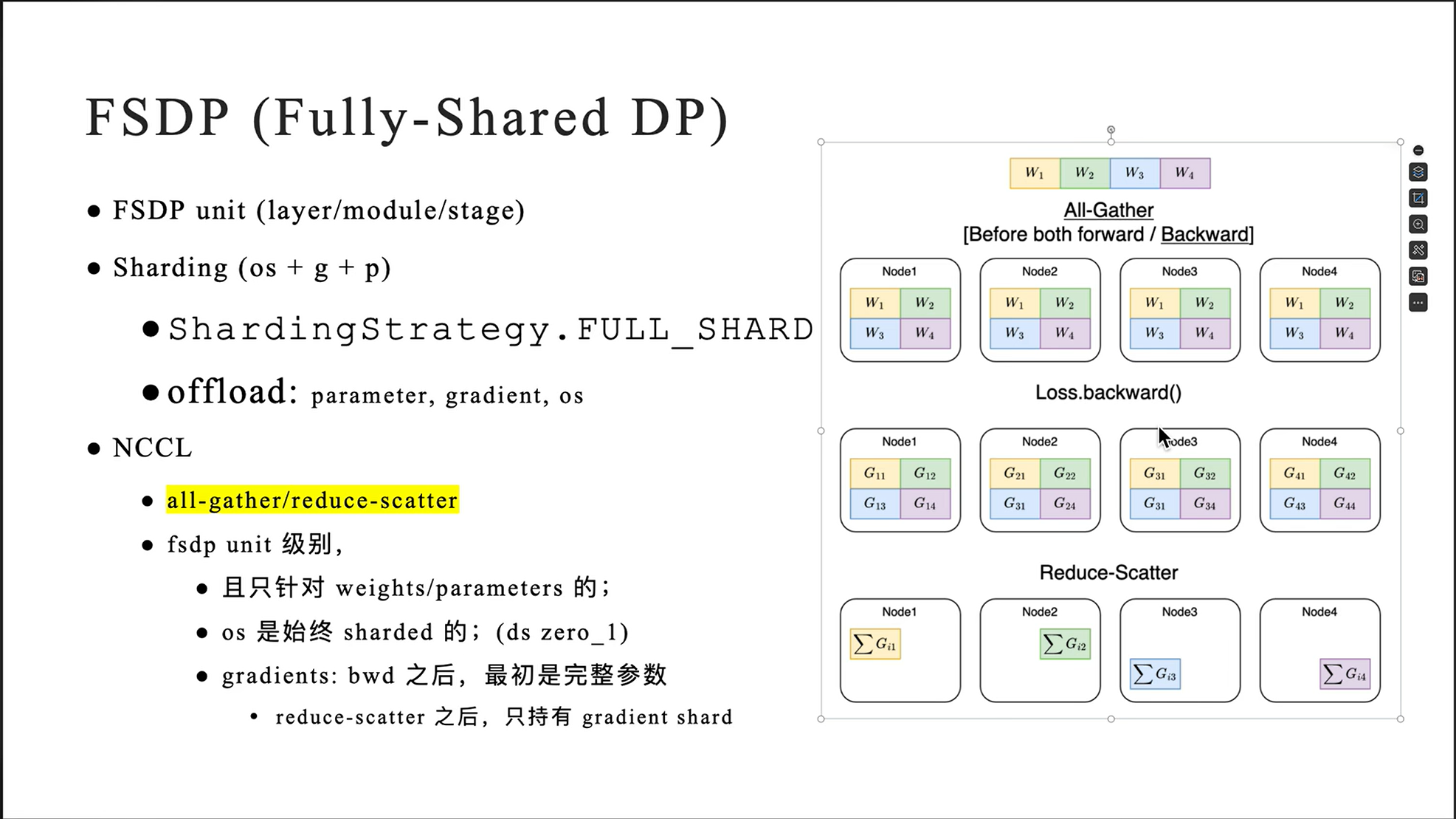
Preliminary：FSDP（Fully Shared DP）

• all-gather/reduce-scatter

from IPython.display import Image

• N 张卡组成一个 ring 环，计算步数，2(N-1)
  • scatter-reduce: (N-1)，非标准 nccl
  • all-gather: (N-1)
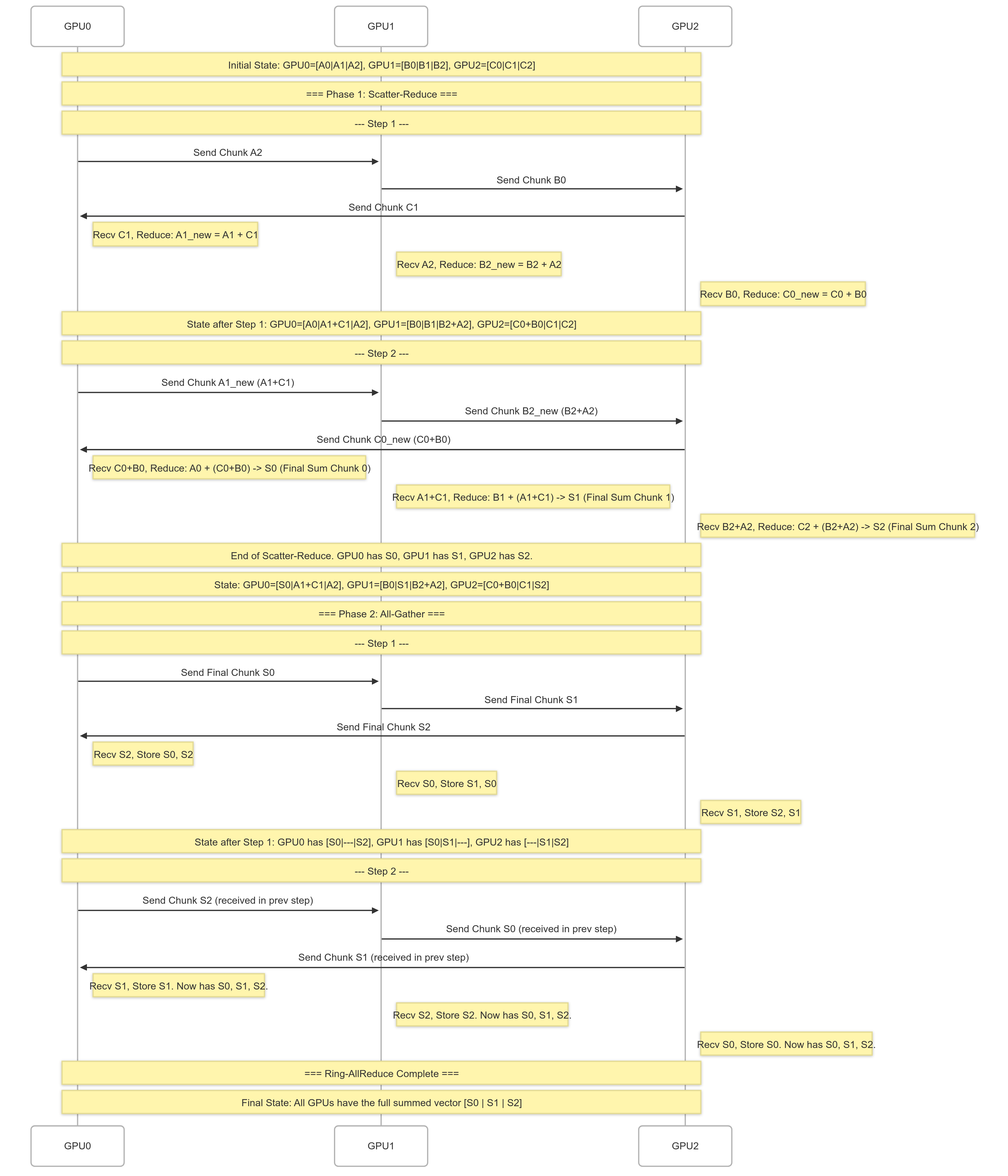
• 3张卡，长度为6的向量加和为例；
  • input (each gpu model gradients):
    • [a0, a1 | a2, a3 | a4, a5] = [A0 | A1 | A2]
    • [b0, b1 | b2, b3 | b4, b5] = [B0 | B1 | B2]
    • [c0, c1 | c2, c3 | c4, c5] = [C0 | C1 | C2]
  • output (sync model gradients across gpus):
    • [a0+b0+c0, a1+b1+c1, a2+b2+c2, a3+b3+c3, a4+b4+c4, a5+b5+c5]
    • [A0 + B0 + C0 | A1 + B1 + C1 | A2 + B2 + C2]

这里要做的一个事情就是，三张卡上有三份不同的数据，现在要把它们加和起来并结算到某一张卡上去。

torch scatter reduce

• https://pytorch.org/docs/stable/generated/torch.Tensor.scatter_reduce_.html

import torch

src = torch.tensor([1., 2., 3., 4., 5., 6.])
index = torch.tensor([0, 1, 0, 1, 2, 1])
input = torch.tensor([1., 2., 3., 4.])
input.scatter_reduce(0, index, src, reduce="sum", include_self=True)

1+(1+3), 2+(2+4+6), 3+(5), 4
# tensor([5, 14, 8, 4])

src = torch.tensor([1., 2., 3., 4., 5., 6.])
index = torch.tensor([0, 1, 0, 1, 2, 1])
input = torch.tensor([1., 2., 3., 4.])
input.scatter_reduce(0, index, src, reduce="mean", include_self=True)

(1+(1+3))/3, (2+(2+4+6))/4, (3+(5))/2, 4
# tensor([1.667, 3.5, 4.0, 4])

上面的例子中，source是src = [1,2,3,4,5,6]，然后我们要把这些数据按照index中的索引进行scatter，scatter到input中去，然后做reduce操作（比如求和）

比如0这个位置要进来两个数据（1 和 3），也就是（1+1+3），其他位置是一样的，input里原先的数据也是要算进去的。

phase1： scatter reduce

减少通信量；先分块，以降低通信量，下面介绍的是

• [a0, a1 | a2, a3 | a4, a5] = [A0 | A1 | A2]
• [b0, b1 | b2, b3 | b4, b5] = [B0 | B1 | B2]
• [c0, c1 | c2, c3 | c4, c5] = [C0 | C1 | C2]
• scatter：data chunks，reduce：规约（降维）
  • nccl 是 reduce-scatter
  • 下面两步走是ring-allreduce的一算法
• step1
  • GPU0 =>(A2) GPU1 =>(B0) GPU2 =>(C1) GPU0
    • GPU0: A1 + C1, [A0, A1+C1, A2]
    • GPU1: B2 + A2, [B0, B1, B2+A2]
    • GPU2: C0 + B0, [C0+B0, C1, C2]
• step2
  • GPU0 =>(A1+C1) GPU1 =>(B2+A2) GPU2 =>(C0+B0) GPU0
    • GPU0: [C0+B0+A0, A1+C1, A2]
    • GPU1: [B0, A1+C1+B1, B2+A2]
    • GPU2: [C0+B0, C1, B2+A2+C2]

上面就是第一轮一个环状的传数据，第二轮也是环状传数据三张卡，第一轮只传了一个块，第二轮就两个块，两轮结束，需要计算的所有数据都有了，然后就是reduce/gather到一张卡上。

phase2: all-gather

gather再两步，就三张卡都有需要的数据了。

• S0: A0+B0+C0, S1: A1+B1+C1, S2: A2+B2+C2
• step1:
  • GPU0 =>(S0) GPU1 =>(S1) GPU2 =>(S2) GPU0
    • GPU0: [S0, …, S2]
    • GPU1: [S0, S1, …]
    • GPU2: […, S1, S2]
• step2:
  • GPU0 =>(S2) GPU1 =>(S0) GPU2 =>(S1) GPU0
    • GPU0: [S0, S1, S2]
    • GPU1: [S0, S1, S2]
    • GPU2: [S0, S1, S2]

下面是对上面两步走操作的图示例：

why ring-allreduce

• 高效的带宽利用率 (Efficient Bandwidth Utilization):
  • 分块传输: Ring-AllReduce 将需要同步的数据（例如梯度）分成多个小块（chunks）。
  • 流水线效应: 数据块在环上逐步传输和计算。一个 GPU 可以同时发送一个块给下一个节点，并从上一个节点接收另一个块。这种流水线方式使得 GPU 间的通信链路（如 NVLink 或网络带宽）能够持续被利用，而不是在等待整个大块数据传输完成。
  • 点对点通信: 每个 GPU 只需与其在环中的直接邻居通信。这使得算法可以充分利用现代 GPU 系统中高速的点对点连接（如 NVLink），避免了所有 GPU 都向一个中心点发送数据可能造成的拥塞。理论上，在 N 个 GPU 的环中，每个 GPU 在 Scatter-Reduce 和 All-Gather 阶段总共发送和接收的数据量大约是 2 * (N-1)/N * TotalDataSize，接近于最优值 2 * TotalDataSize。
• 均衡的通信负载 (Balanced Communication Load):
  • 在 Ring-AllReduce 中，每个 GPU 发送和接收的数据量大致相同，计算负载（Reduce 操作）也相对均衡地分布在各个步骤中。
  • 这避免了像基于树（Tree-based）的 All-Reduce 算法中可能出现的根节点通信瓶颈问题，因为在树形结构中，靠近根节点的 GPU 需要处理更多的数据聚合或分发任务。
• 避免中心瓶颈 (Avoids Central Bottleneck):
  • 与参数服务器（Parameter Server）架构或其他需要中心协调节点的同步方法不同，Ring-AllReduce 是完全去中心化的。没有单个节点会成为性能瓶颈或单点故障。
• 良好的可扩展性 (Good Scalability):
  • 虽然完成一次完整的 Ring-AllReduce 需要 2 * (N-1) 步（N 是 GPU 数量），延迟会随着 N 线性增加，但关键在于每个 GPU 的带宽需求基本保持不变（与 N 无关）。
    对于带宽是主要瓶颈的大规模系统（尤其是在传输大量梯度时），这种恒定的带宽需求使得 Ring-AllReduce 比那些带宽需求随节点数增加而增加的算法更具扩展性。

---

FSDP回顾

https://www.bilibili.com/BV1Kx4y187Te

---

[Pytorch 分布式] DeepSpeed Ulysses 分布式序列并行算法，尤利西斯，Ring attention

video
code

长上下文的计算复杂度是$O(n^2)$的，这是个很糟糕的复杂度。

• 优化长序列（long sequence，1M context window）的问题；
  • DP, TP, PP & SP
  • 长序列拆分到不同的设备上计算，每个设备处理 sub seq；
• https://arxiv.org/pdf/2105.13120
  • Sequence Parallelism: Long Sequence Training from System Perspective
• https://arxiv.org/pdf/2309.14509
  • DeepSpeed Ulysses: System Optimizations for Enabling Training of Extreme Long Sequence Transformer Models

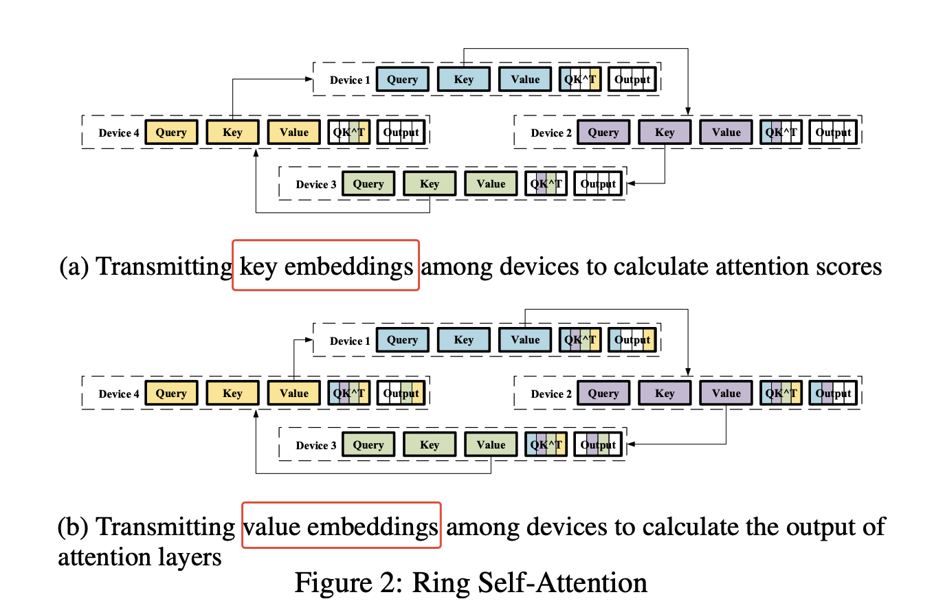
Ring Attention

• Ring-AllReduce：通信换内存

  • 序列 split/shard 到多张卡上，即每张卡只保存一个 sub seq；
  • (Ring)QK & (Ring)AV
    • 每个 device sub seq 的 Query 需要跟其他 devices 上的所有的 Key 做计算；
      $$\text{Attention}(Q,K,V)=\underset{\mathbf{A}}{\underbrace{\text{softmax}\left(\frac{Q{K}^{\top }}{\sqrt{d_k}}\right)}}V$$

• N 个 devices，N-1 次 iter，每个 device 都有完整的 QK^T 的结果

$$\underset{\begin{array}{c}\uparrow \\ (b,n,d_v)\end{array}}{\text{Attention}(Q,K,V)}=\underset{\text{Weights Dim: }(b,n,n)}{\underbrace{\text{softmax}\left(\frac{\stackrel{\text{Scores Dim: }(b,n,n)}{\overbrace{\underset{\begin{array}{c}\uparrow \\ (b,n,d_k)\end{array}}{Q}\cdot \underset{\begin{array}{c}\uparrow \\ (b,d_k,n)\end{array}}{K^T}}}}{\underset{\begin{array}{c}\uparrow \\ \text{scalar}\end{array}}{\sqrt{d_k}}}\right)}}\cdot \underset{\begin{array}{c}\uparrow \\ (b,n,d_v)\end{array}}{V}$$

DeepSpeed UIysses

这张图来自https://arxiv.org/pdf/2309.14509

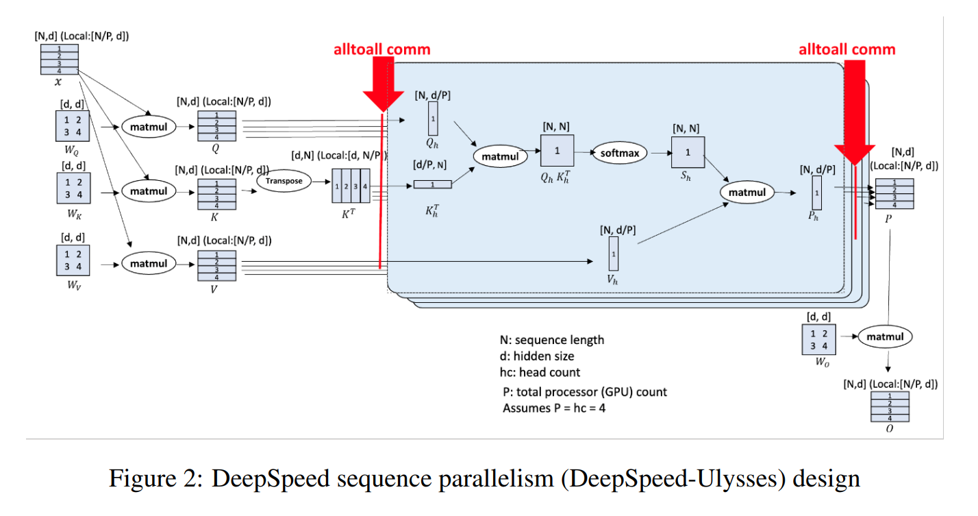
• Ulysses：尤利西斯（a very long novel)；
• all-to-all communication collective
  • DeepSpeed-Ulysses partitions individual samples along the sequence dimension among participating GPUs.
  • Then right before the attention computation, it employs all-to-all communication collective on the partitioned queries, keys and values such that each GPU receives the full sequence but only for a non-overlapping subset of the attention heads. This allows the participating GPUs to compute attention for different attention heads in parallel.
    • gather_seq_scatter_heads
  • Finally, DeepSpeed-Ulysses employs another all-to-all to gather the results along the attention heads while re-partitioning along the sequence dimension.
    • gather_heads_scatter_seq
• 将输入序列 X (长度 N) 沿序列维度切分为 SP 块，每个 GPU 分配到 N/SP 长度的子序列。
  • 对于非注意力层 (如 MLP)，计算是完全局部的，每个 GPU 处理自己的子序列即可。
    • token 之间独立，token-level projection
    • Ulysses SP的核心复杂性在于Attention层。为了让每个token在计算注意力时能够考虑到全局序列信息（或者说，让每个head在计算时能看到完整的序列，即使这个head只在当前rank计算），Attention模块前后需要进行两次精密的all-to-all数据重排。MLP层则没有这样的需求，数据在进入MLP时已经是按序列分片好的，可以直接进行本地计算。
  • 对于注意力层:
    • 步骤 1 (计算 Q, K, V): 每个 GPU 基于其本地子序列计算出本地的 Q_local, K_local, V_local (维度约为 N/SP x d，d 是隐藏维度)。
    • 步骤 2 (全局 K, V 收集 - 关键): 使用 All-to-All 通信操作（All-Gather??）。每个 GPU 将自己的 K_local, V_local 发送给所有其他 GPU，并接收来自所有其他 GPU 的 K, V 块。执行后，每个 GPU 拥有完整的全局 K 和 V 矩阵 (维度 N x d)，但仍然只拥有本地的 Q_local (维度 N/SP x d)。
      • https://docs.nvidia.com/deeplearning/nccl/user-guide/docs/usage/collectives.html
    • 步骤 3 (本地注意力计算): 每个 GPU 使用其 Q_local 和完整的全局 K, V 计算其负责的那部分注意力输出 O_local (维度 N/SP x d)。计算公式为 Attention(Q_local, K_global, V_global)。这一步的计算量是 (N/SP) * N * d，内存瓶颈在于存储临时的注意力分数矩阵，大小约为 (N/SP) * N。相比原始的 N*N，内存显著降低。
    • 步骤 4 (可选的输出重组): 如果后续层需要按序列拼接的完整输出，可能需要另一次通信（如 All-Gather 或另一次 All-to-All 的变种）来组合 O_local。但在 DeepSpeed 实现中，通常保持分布式状态，直接输入到下一个同样按序列并行的层。

verl sp

verl源码中在./models/transformers/monkey_patch.py中有对fsdp这个的详细实现：

• torchrun --nproc_per_node=2 -m pytest tests/model/test_transformers_ulysses.py -svv
  • dp_size = world_size // sp_size
• monkey_patch
  • _flash_attention_forward => _ulysses_flash_attention_forward
  • 假设序列并行数 ulysses_sp_size = N。每个SP rank最初拥有 (batch_size, seq_len / N, num_heads, head_dim) 形状的 Q, K, V 张量。
    • gather_seq_scatter_heads
      • [bsz, seq/n, h, ...] -> [bsz, seq, h/n, ...] （for Q/K/V）
        • 得到完整的序列，部分的头；
    • flash-attn => [bsz, seq, h/n, ...]
    • gather_heads_scatter_seq
      • [bsz, seq, h/n, ...] -> [bsz, seq/n, h, ...]
        • 得到部分的序列，完整的头；
• 数据并行（fsdp）与 sp
  • fsdp：优化的是模型参数所占显存，sp：优化的是激活所占显存
  • fsdp: all-gather, reduce-scatter
  • sp: all-to-all

      SP=4 (列) -->
DP=2  GPU(0,0) GPU(0,1) GPU(0,2) GPU(0,3)  <-- DP Group 0 (Row 0)
(行)  GPU(1,0) GPU(1,1) GPU(1,2) GPU(1,3)  <-- DP Group 1 (Row 1)
 |
 V

import torch
import torch.nn.functional as F

# --- 参数设定 ---
batch_size = 1
seq_len = 12  # 总序列长度
d_model = 8   # 嵌入维度 (为了清晰起见保持较小)
num_devices = 3 # 模拟的设备/分块数量
chunk_len = seq_len // num_devices # 每个设备上的序列块长度

assert seq_len % num_devices == 0, "序列长度必须能被设备数量整除"

Q = torch.randn(batch_size, seq_len, d_model)
K = torch.randn(batch_size, seq_len, d_model)
V = torch.randn(batch_size, seq_len, d_model)

scale = d_model ** -0.5 # 缩放因子
# 计算注意力分数: Q @ K^T
attn_scores_standard = torch.matmul(Q, K.transpose(-2, -1)) * scale
# 应用 Softmax 获取注意力权重
attn_weights_standard = F.softmax(attn_scores_standard, dim=-1)
# 将权重应用于 V 得到输出
output_standard = torch.matmul(attn_weights_standard, V)

output_standard.shape # torch.Size([1, 12, 8])

ring sa

Q_chunks = list(torch.chunk(Q, num_devices, dim=1))
K_chunks = list(torch.chunk(K, num_devices, dim=1))
V_chunks = list(torch.chunk(V, num_devices, dim=1))

print(f"Q 被切分成 {len(Q_chunks)} 块, 每块形状: {Q_chunks[0].shape}")
print(f"K 被切分成 {len(K_chunks)} 块, 每块形状: {K_chunks[0].shape}")
print(f"V 被切分成 {len(V_chunks)} 块, 每块形状: {V_chunks[0].shape}")

输出：

Q 被切分成 3 块, 每块形状: torch.Size([1, 4, 8])
K 被切分成 3 块, 每块形状: torch.Size([1, 4, 8])
V 被切分成 3 块, 每块形状: torch.Size([1, 4, 8])

# --- 2. Ring Self-Attention Simulation ---
print("\n--- Simulating Ring Self-Attention ---")

# Split tensors into chunks for each "device"
Q_chunks = list(torch.chunk(Q, num_devices, dim=1))
K_chunks = list(torch.chunk(K, num_devices, dim=1))
V_chunks = list(torch.chunk(V, num_devices, dim=1))

print(f"Split Q into {len(Q_chunks)} chunks, each shape: {Q_chunks[0].shape}")
print(f"Split K into {len(K_chunks)} chunks, each shape: {K_chunks[0].shape}")
print(f"Split V into {len(V_chunks)} chunks, each shape: {V_chunks[0].shape}")

output_chunks_rsa = []

# Simulate computation on each device
for i in range(num_devices):
    print(f"\n-- Simulating Device {i} --")
    q_local = Q_chunks[i] # Query chunk for this device
    ordered_scores = [None] * num_devices

    # Ring communication for Keys
    print(f"  Device {i} Q shape: {q_local.shape}")
    for j in range(num_devices):
        k_idx = (i - j + num_devices) % num_devices # Index of K chunk received in this step
        k_remote = K_chunks[k_idx]
        print(f"  Step {j}: Device {i} using K chunk from Device {k_idx} (Shape: {k_remote.shape})")

        # Calculate partial attention scores: Q_local @ K_remote^T
        scores_part = torch.matmul(q_local, k_remote.transpose(-2, -1)) * scale
        print(f"    Partial scores shape for K_{k_idx}: {scores_part.shape}")
        ordered_scores[k_idx] = scores_part

    # Concatenate partial scores in the correct order (k=0, 1, ..., N-1)
    all_scores_for_q_i = torch.cat(ordered_scores, dim=-1)
    print(f"  Device {i}: Concatenated scores shape (Correct Order): {all_scores_for_q_i.shape}") # Should be [batch, chunk_len, seq_len]

    # Apply Softmax
    attn_weights_for_q_i = F.softmax(all_scores_for_q_i, dim=-1)
    print(f"  Device {i}: Softmax weights shape: {attn_weights_for_q_i.shape}")

    # Apply weights to Value matrix (using reconstructed full V for equivalence check)
    full_V = torch.cat(V_chunks, dim=1) # Reconstruct full V for calculation
    output_chunk_i = torch.matmul(attn_weights_for_q_i, full_V)
    print(f"  Device {i}: Output chunk shape: {output_chunk_i.shape}") # Should be [batch, chunk_len, d_model]

    output_chunks_rsa.append(output_chunk_i)

输出：

--- Simulating Ring Self-Attention ---
Split Q into 3 chunks, each shape: torch.Size([1, 4, 8])
Split K into 3 chunks, each shape: torch.Size([1, 4, 8])
Split V into 3 chunks, each shape: torch.Size([1, 4, 8])

-- Simulating Device 0 --
  Device 0 Q shape: torch.Size([1, 4, 8])
  Step 0: Device 0 using K chunk from Device 0 (Shape: torch.Size([1, 4, 8]))
    Partial scores shape for K_0: torch.Size([1, 4, 4])
  Step 1: Device 0 using K chunk from Device 2 (Shape: torch.Size([1, 4, 8]))
    Partial scores shape for K_2: torch.Size([1, 4, 4])
  Step 2: Device 0 using K chunk from Device 1 (Shape: torch.Size([1, 4, 8]))
    Partial scores shape for K_1: torch.Size([1, 4, 4])
  Device 0: Concatenated scores shape (Correct Order): torch.Size([1, 4, 12])
  Device 0: Softmax weights shape: torch.Size([1, 4, 12])
  Device 0: Output chunk shape: torch.Size([1, 4, 8])

-- Simulating Device 1 --
  Device 1 Q shape: torch.Size([1, 4, 8])
  Step 0: Device 1 using K chunk from Device 1 (Shape: torch.Size([1, 4, 8]))
    Partial scores shape for K_1: torch.Size([1, 4, 4])
  Step 1: Device 1 using K chunk from Device 0 (Shape: torch.Size([1, 4, 8]))
    Partial scores shape for K_0: torch.Size([1, 4, 4])
  Step 2: Device 1 using K chunk from Device 2 (Shape: torch.Size([1, 4, 8]))
    Partial scores shape for K_2: torch.Size([1, 4, 4])
  Device 1: Concatenated scores shape (Correct Order): torch.Size([1, 4, 12])
  Device 1: Softmax weights shape: torch.Size([1, 4, 12])
  Device 1: Output chunk shape: torch.Size([1, 4, 8])

-- Simulating Device 2 --
  Device 2 Q shape: torch.Size([1, 4, 8])
  Step 0: Device 2 using K chunk from Device 2 (Shape: torch.Size([1, 4, 8]))
    Partial scores shape for K_2: torch.Size([1, 4, 4])
  Step 1: Device 2 using K chunk from Device 1 (Shape: torch.Size([1, 4, 8]))
    Partial scores shape for K_1: torch.Size([1, 4, 4])
  Step 2: Device 2 using K chunk from Device 0 (Shape: torch.Size([1, 4, 8]))
    Partial scores shape for K_0: torch.Size([1, 4, 4])
  Device 2: Concatenated scores shape (Correct Order): torch.Size([1, 4, 12])
  Device 2: Softmax weights shape: torch.Size([1, 4, 12])
  Device 2: Output chunk shape: torch.Size([1, 4, 8])

# Concatenate the output chunks from all devices
output_rsa = torch.cat(output_chunks_rsa, dim=1) # Concatenate along the sequence dimension
print("\n--- RSA Result ---")
print("RSA Concatenated Output Shape:", output_rsa.shape)

# --- 3. Comparison ---
print("\n--- Comparison ---")
# Check if the results are numerically close
are_close = torch.allclose(output_standard, output_rsa, atol=1e-6) # Use a tolerance

print(f"Are Standard Attention and Ring Attention outputs equivalent? {are_close}")

# Verify the shapes match
assert output_standard.shape == output_rsa.shape, "Shapes do not match!"
if are_close:
    print("Success: The Ring Self-Attention simulation produced the same result as standard attention.")
else:
    print("Failure: The results differ.")
    # Optional: Print difference magnitude if they differ
    # diff = torch.abs(output_standard - output_rsa).max()
    # print(f"Maximum absolute difference: {diff.item()}")

输出：

--- RSA Result ---
RSA Concatenated Output Shape: torch.Size([1, 12, 8])

--- Comparison ---
Are Standard Attention and Ring Attention outputs equivalent? True
Success: The Ring Self-Attention simulation produced the same result as standard attention.