Python数据可视化详解（1/5）

matplotlib显示中文与负号

matplotlib.rcParams["font.sans-serif"] = ["SimHei"]
matplotlib.rcParams["axes.unicode_minus"] = False

• Figure 对象

import matplotlib.pyplot as plt
import numpy as np

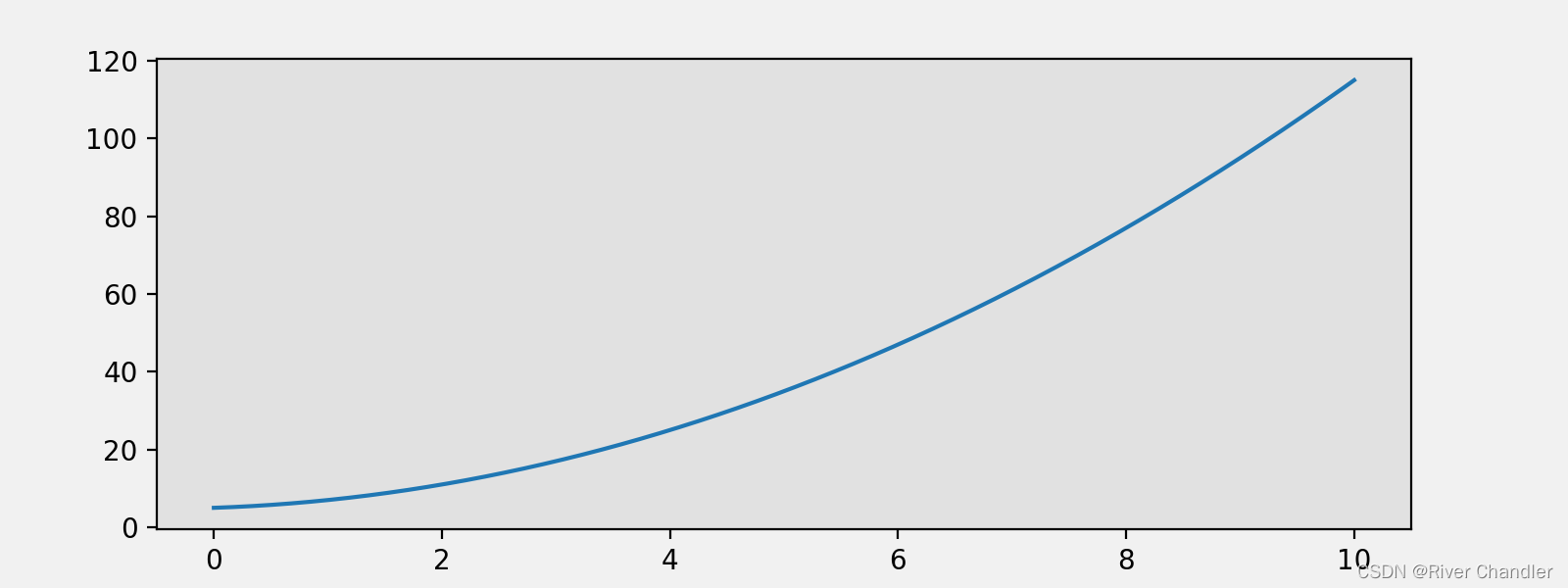
x = np.arange(0,10.01,0.01)
y = x**2 + x + 5

fig = plt.figure(figsize=(8,3),facecolor="#f1f1f1")
left,bottom,width,height = 0.1,0.1,0.8,0.8
ax = fig.add_axes((left,bottom,width,height),facecolor="#e1e1e1")
ax.plot(x,y)
fig.savefig("0.png",dpi=200,facecolor="#f1f1f1")

Axes 对象

绘图类型

axes.plot	axes.step	axes.bar	axes.hist
折线图	阶梯图	柱状图	直方图

axes.errorbar	axes.scatter	axes.fill_between	axes.quiver
误差棒	点图	区间图	向场

•  

  关键字参数

color	颜色
alpha	透明度(0-1)
linewidth/lw	线宽
linestyle/ls	-实线 --虚线 :点线 .-点画线
marker	+十字形 o圆形 *星形 s方形 .点 1 2 3 4 不同朝向的三角形
marksize
markerfacecolor
markeredgewidth
markeredgecolor

图例

ax.legend(ncol=4,loc=3,bbox_to_anchor=(0,1))

ncol	标签排列成的列数
loc	loc=1  右上 loc=2  左上 loc=3  左下 loc=4  右下
bbox_to_anchor	(x,y) 坐标

文本注释

axes.test  set_title  set_xlabel  set_ylabel axes.annotate

fontsize	字号
family	字体
backgroundcolor	文本标签的背景颜色
color	文本颜色
alpha	透明度
notation	旋转角度

轴属性

轴范围

set_xlim
set_ylim
axis	"tight"   坐标的范围紧密匹配绘制 "equal"   坐标轴的单位长度包含相同的像素点

轴刻度

set_xticks
set_yticks
set_xticklabels
set_yticklabels
grid	格子
对数坐标	loglog 对x,y轴同时使用对数坐标 semilogx  x轴对数坐标 semilogy  y轴对数坐标

双轴图

twinx	共享x轴
twiny	共享y轴

import matplotlib.pyplot as plt
import numpy as np

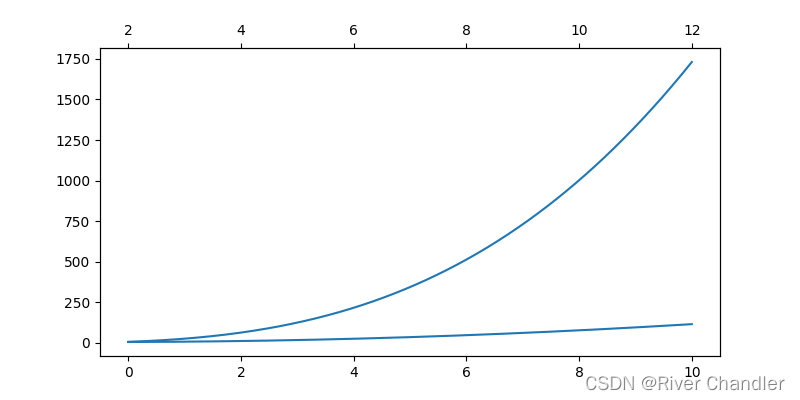
x1 = np.arange(0,10.01,0.01)
y1 = x1**2 + x1 + 5

x2 = np.arange(2,12.01,0.01)
y2 = x2**3 + x2*0.5 - 3

fig,ax1 = plt.subplots(figsize=(8,4))

ax1.plot(x1,y1)
ax2 = ax1.twiny()
ax2.plot(x2,y2)

plt.show()

边框

spines	设置类同上  示例如下
set_position

import matplotlib.pyplot as plt
import numpy as np

x1 = np.arange(0,10.01,0.01)
y1 = x1**2 + x1 + 5

x2 = np.arange(2,12.01,0.01)
y2 = x2**3 + x2*0.5 - 3

fig,ax1 = plt.subplots(figsize=(8,4))

ax1.spines["right"].set_alpha(0.45)
ax1.spines["bottom"].set_linewidth(3)
ax1.spines["left"].set_color("red")
ax1.spines["top"].set_linestyle("-.")


plt.show()

• 操作详解

• 1.pyplot.subplots选项

nrows	子图的行数
ncols	子图的列数
sharex	所有的子图使用相同的x轴刻度
sharey	所有的子图使用相同的y轴刻度

import matplotlib.pyplot as plt

fig = plt.figure()

#add_subplot 创建一个或多个子图

ax1 = fig.add_subplot(2,2,1)

plt.plot([1,2,3,4,5,6,7,8,9,10],[23,43,54,32,34,45,39,43,45,49],"k.-")

ax2 = fig.add_subplot(2,2,2)

ax3 = fig.add_subplot(2,2,3)

plt.plot([1,2,3,4,5,6,7,8,9,10],[23,43,54,32,34,45,39,43,45,49],"k--")

########只对最后一个创建的图起作用

plt.show()

• 2.颜色，标记、线类型和图例

plot参数
linestyle=	figure	linestyle=	figure
“--”	虚线	“dashdot”
“-”	实线	“dotted”
“-.”		“None”
“solid”		“:”	通过点线连接数据点
scatter参数
marker
"o"	空心圆圈	"."
label		plt.legend(loc=”best”)   保存在最合适的位置

import matplotlib.pyplot as plt

plt.plot([1,2,3,4],[2,3,4,5],linestyle="-.",color="green",label="this is the line")

plt.plot([2,3,4,6,7],[2,3,4,5,3],label="this is different")

plt.legend()

plt.savefig("None")

• 3.刻度和标签

在数据范围内设定刻度的位置	set_xticks()
为标签赋值(比如原来用厘米表示的长度单位可以简化为用米表示)	set_xticklabels()
将x轴刻度标签旋转	rotation=
添加标题	set_xlabel()
x轴y轴相同
x轴的极限	xlimit()

import matplotlib.pyplot as plt
import random

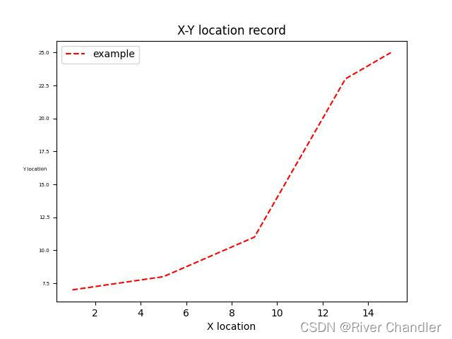
x = [1,5,9,13,15]
y = [7,8,11,23,25]

plt.xlabel("X location")
plt.ylabel("Y location",rotation=True,fontsize=5)
plt.title("X-Y location record")

plt.xticks(fontsize=10)
plt.yticks(fontsize=5)

plt.plot(x,y,linestyle="--",color="r",label="example")
plt.legend()
plt.savefig("0.jpg")

• 4.注释与子图加工

text(x,y，“注释”，fontsize=10）
x,y添加注释的位置	一个字符串	字体大小
annotate(label,xy=(坐标),xytext=（注释位置)，arrowprops=dict（headwidth=4，headlength=4 ））	添加箭头

• 5.图片的保存

参数
fname	文件名
dpi	分辨率
facecolor	背景颜色
format	文件格式
Bbox_inches	若等于“tight”，将去掉周围空白部分

import matplotlib.pyplot as plt

plt.plot([2,3,4,7,8],[45,43,34,43,23])
plt.savefig(fname="l.pdf",dpi=10000,facecolor="green",format="pdf")
plt.savefig(fname="j.pdf",dpi=10000,facecolor="green",format="pdf",bbox_inches="tight")
plt.savefig(fname="lj.pdf",dpi=10000,format="pdf",bbox_inches="tight")

• 6.对数坐标

plt.semilogy([2,4,8,16,32],[1,10,100,1000,10000])
plt.show()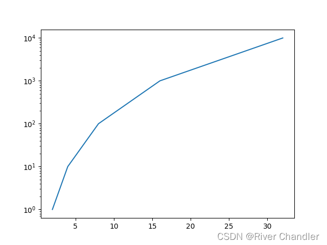

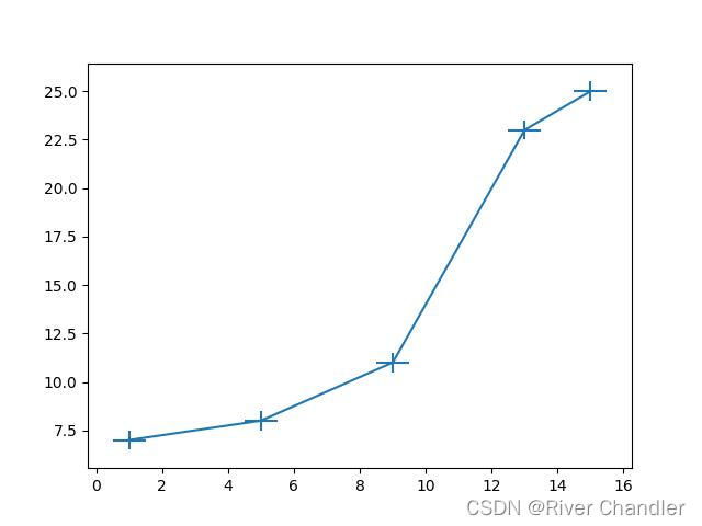
• 7.误差棒

import matplotlib.pyplot as plt
import random

x = [1,5,9,13,15]
y = [7,8,11,23,25]
x_errors = 0.5
y_errors = 0.5

plt.errorbar(x,y,yerr=y_errors,xerr=x_errors)

plt.savefig("0.jpg")

 

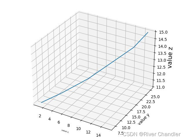
•  8.3D图形

import matplotlib.pyplot as plt
from mpl_toolkits.mplot3d import Axes3D

fig = plt.figure()
ax = Axes3D(fig)
x = [1,5,9,13,15]
y = [7,8,11,23,25]
z = [11,12,13,14,15]
ax.plot(x,y,z)

plt.xlabel("value x",rotation=True,fontsize=5)
plt.ylabel("value y",rotation=True,fontsize=10)
ax.set_zlabel("value z",rotation=True,fontsize=15)

plt.savefig("0.jpg")

• 9. 多重绘图
  • 统一坐标轴上的多重绘图

import matplotlib.pyplot as plt
x1 = [1,2,3,4]
x2 = [1,2,5,6]
y1 = [4,5,6,9]
y2 = [5,8,9,9]
plt.plot(x1,y1,x2,y2)
plt.show()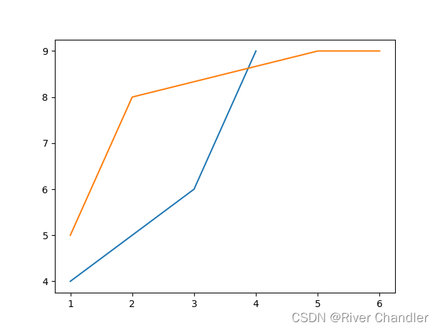

•   
  • 替换曲线
    • plt.cla()  清除坐标轴命令
• 子绘图
  • plt.subplot(M,N,p)  将图形窗口按M行N列的网格分割 设置p个子区域为激活

plt.subplot(3,4,2)
plt.plot([4,3,2,1],[1,2,3,4])
plt.show()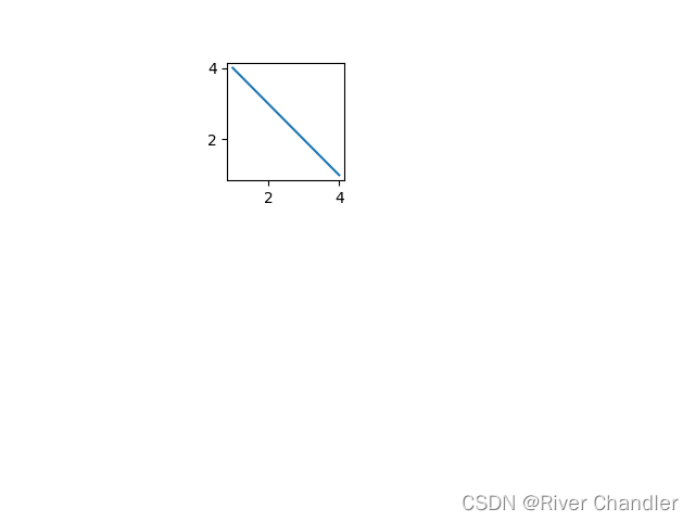

实例 Python 绘制格罗春图

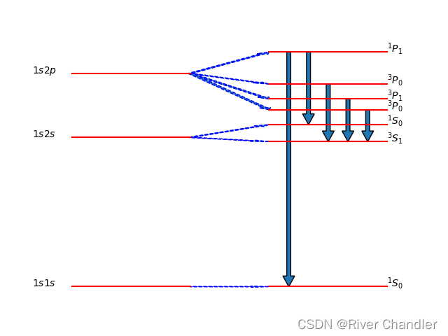
import matplotlib.pyplot as plt
plt.cla()
config = [[1,0,""],[1,7,""],[1,10,""]]
fine_level = [[2,11,r'$^1P_1$'],[2,9.5,r'$^3P_0$'],
              [2,8.8,r'$^3P_1$'],[2,8.3,r'$^3P_0$'],[2,7.6,r'$^1S_0$'],[2,6.8,r'$^3S_1$'],
              [2,0,r'$^1S_0$']]

energy_point = config + fine_level
plt.axis("off")
for each_point in energy_point:
    start = [each_point[0]-0.3,each_point[0]+0.3]
    stop = [each_point[1],each_point[1]]
    plt.plot(start,stop,color="r")
    plt.text(each_point[0]+0.3,
             each_point[1],each_point[2])
DY = [[0],[0.6,-0.2],[1,-0.5,-1.2,-1.7]]
DX = 0.4
i = 0
for each_config in config:
    x = each_config[0]
    y = each_config[1]
    Dys = DY[i]
    for each_dy in Dys:
        plt.arrow(x+0.3,y,DX,each_dy,width=0.02,
                  length_includes_head=True,ec="blue",ls="dashed")
    i += 1
        
plt.text(0.5,0,r'$1s1s$')
plt.text(0.5,7,r'$1s2s$')
plt.text(0.5,10,r'$1s2p$')

plt.arrow(2-0.2,11,0,-11,width=0.02,
          length_includes_head=True,head_length=0.5,ec="black")
plt.arrow(2-0.1,11,0,-3.4,width=0.02,
          length_includes_head=True,head_length=0.5,ec="black")
plt.arrow(2,9.5,0,-2.7,width=0.02,
          length_includes_head=True,head_length=0.5,ec="black")
plt.arrow(2.1,8.8,0,-2.0,width=0.02,
          length_includes_head=True,head_length=0.5,ec="black")
plt.arrow(2.2,8.3,0,-1.5,width=0.02,
          length_includes_head=True,head_length=0.5,ec="black")