决策树--从原理到实现

================================================================================

算算有相当一段时间没写blog了，主要是这学期作业比较多，而且我也没怎么学新的东西

接下来打算实现一个小的toy lib：DML，同时也回顾一下以前学到的东西

当然我只能保证代码的正确性，不能保证其效率啊~~~~~~

之后我会陆续添加进去很多代码，可以供大家学习的时候看，实际使用还是用其它的吧

================================================================================

一.引入

决策树基本上是每一本机器学习入门书籍必讲的东西，其决策过程和平时我们的思维很相似，所以非常好理解，同时有一堆信息论的东西在里面，也算是一个入门应用，决策树也有回归和分类，但一般来说我们主要讲的是分类，方便理解嘛。

虽然说这是一个很简单的算法，但其实现其实还是有些烦人，因为其feature既有离散的，也有连续的，实现的时候要稍加注意

          (不同特征的决策，图片来自【1】)

O-信息论的一些point：

     首先看这里： http://blog.csdn.net/dark_scope/article/details/8459576

             然后加入一个叫信息增益的东西：

             □.信息增益：(information gain)

                                 g(D,A) = H(D)-H(D|A)

                                 表示了特征A使得数据集D的分类不确定性减少的程度

             □.信息增益比：(information gain ratio)

                                  g‘(D,A)=g(D,A) / H(D)

             □.基尼指数：

             

                        

                         

二.各种算法

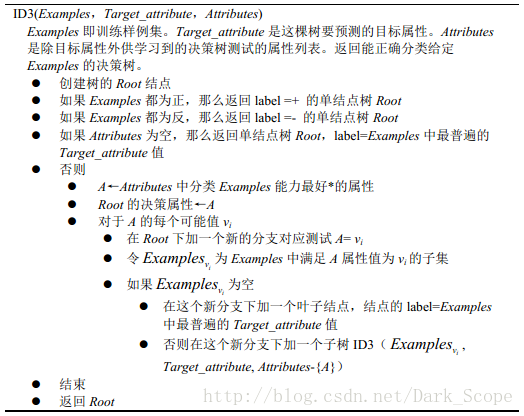
1.ID3

ID3算法就是对各个feature信息计算信息增益，然后选择信息增益最大的feature作为决策点将数据分成两部分

                然后再对这两部分分别生成决策树。

                 图自【1】

       

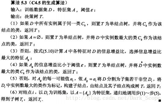
2.C4.5

                C4.5与ID3相比其实就是用信息增益比代替信息增益，应为信息增益有一个缺点：

                       信息增益选择属性时偏向选择取值多的属性

                算法的整体过程其实与ID3差异不大：图自【2】

                 

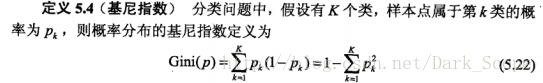
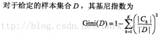
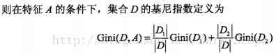
3.CART

CART(classification and regression tree)的算法整体过程和上面的差异不大，然是CART的决策是二叉树的

每一个决策只能是“是”和“否”，换句话说，即使一个feature有多个可能取值，也只选择其中一个而把数据分类

两部分而不是多个，这里我们主要讲一下分类树，它用到的是基尼指数：

图自【2】

三.代码及实现

                  好吧，其实我就想贴贴代码而已……本代码在https://github.com/justdark/dml/tree/master/dml/DT

                  纯属toy~~~~~实现的CART算法：

                 

from __future__ import division
import numpy as np
import scipy as sp
import pylab as py
def pGini(y):
		ty=y.reshape(-1,).tolist()
		label = set(ty)
		sum=0
		num_case=y.shape[0]
		#print y
		for i in label:
			sum+=(np.count_nonzero(y==i)/num_case)**2
		return 1-sum
	
class DTC:
	def __init__(self,X,y,property=None):
		'''
			this is the class of Decision Tree
			X is a M*N array where M stands for the training case number
								   N is the number of features
			y is a M*1 vector
			property is a binary vector of size N
				property[i]==0 means the the i-th feature is discrete feature,otherwise it's continuous
				in default,all feature is discrete
				
		'''
		'''
			I meet some problem here,because the ndarry can only have one type
			so If your X have some string parameter,all thing will translate to string
			in this situation,you can't have continuous parameter
			so remember:
			if you have continous parameter,DON'T PUT any STRING IN X  !!!!!!!!
		'''
		self.X=np.array(X)
		self.y=np.array(y)
		self.feature_dict={}
		self.labels,self.y=np.unique(y,return_inverse=True)
		self.DT=list()
		if (property==None):
			self.property=np.zeros((self.X.shape[1],1))
		else:
			self.property=property
			
		for i in range(self.X.shape[1]):
			self.feature_dict.setdefault(i)
			self.feature_dict[i]=np.unique(X[:,i])

		if (X.shape[0] != y.shape[0] ):
			print "the shape of X and y is not right"
			
		for i in range(self.X.shape[1]):
			for j in self.feature_dict[i]:
				pass#print self.Gini(X,y,i,j)
		pass

	def Gini(self,X,y,k,k_v):
		if (self.property[k]==0):
			#print X[X[:,k]==k_v],'dasasdasdasd'
			#print X[:,k]!=k_v
			c1 = (X[X[:,k]==k_v]).shape[0]
			c2 = (X[X[:,k]!=k_v]).shape[0]
			D = y.shape[0]
			return c1*pGini(y[X[:,k]==k_v])/D+c2*pGini(y[X[:,k]!=k_v])/D
		else:
			c1 = (X[X[:,k]>=k_v]).shape[0]
			c2 = (X[X[:,k]<k_v]).shape[0]
			D = y.shape[0]
			#print c1,c2,D
			return c1*pGini(y[X[:,k]>=k_v])/D+c2*pGini(y[X[:,k]<k_v])/D
		pass
	def makeTree(self,X,y):
		min=10000.0
		m_i,m_j=0,0
		if (np.unique(y).size<=1):

			return (self.labels[y[0]])
		for i in range(self.X.shape[1]):
			for j in self.feature_dict[i]:
				p=self.Gini(X,y,i,j)
				if (p<min):
					min=p
					m_i,m_j=i,j
		
		

		if (min==1):
			return (y[0])
		left=[]
		righy=[]
		if (self.property[m_i]==0):
			left = self.makeTree(X[X[:,m_i]==m_j],y[X[:,m_i]==m_j])
			right = self.makeTree(X[X[:,m_i]!=m_j],y[X[:,m_i]!=m_j])
		else :
			left = self.makeTree(X[X[:,m_i]>=m_j],y[X[:,m_i]>=m_j])
			right = self.makeTree(X[X[:,m_i]<m_j],y[X[:,m_i]<m_j])
		return [(m_i,m_j),left,right]
	def train(self):
		self.DT=self.makeTree(self.X,self.y)
		print self.DT
		
	def pred(self,X):
		X=np.array(X)
		  
		result = np.zeros((X.shape[0],1))
		for i in range(X.shape[0]):
			tp=self.DT
			while ( type(tp) is  list):
				a,b=tp[0]
				
				if (self.property[a]==0):
					if (X[i][a]==b):
						tp=tp[1]
					else:
						tp=tp[2]
				else:
					if (X[i][a]>=b):
						tp=tp[1]
					else:
						tp=tp[2]
			result[i]=self.labels[tp]
		return result
		pass
	

               这个maketree让我想起了线段树………………代码里的变量基本都有说明

试验代码：

  

from __future__ import division
import numpy as np
import scipy as sp
from dml.DT import DTC
X=np.array([
[0,0,0,0,8],
[0,0,0,1,3.5],
[0,1,0,1,3.5],
[0,1,1,0,3.5],
[0,0,0,0,3.5],
[1,0,0,0,3.5],
[1,0,0,1,3.5],
[1,1,1,1,2],
[1,0,1,2,3.5],
[1,0,1,2,3.5],
[2,0,1,2,3.5],
[2,0,1,1,3.5],
[2,1,0,1,3.5],
[2,1,0,2,3.5],
[2,0,0,0,10],
])


y=np.array([
[1],
[0],
[1],
[1],
[0],
[0],
[0],
[1],
[1],
[1],
[1],
[1],
[1],
[1],
[1],
])
prop=np.zeros((5,1))
prop[4]=1
a=DTC(X,y,prop)
a.train()
print a.pred([[0,0,0,0,3.0],[2,1,0,1,2]])

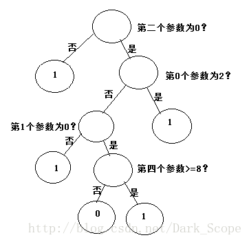
可以看到可以学习出一个决策树：

展示出来大概是这样：注意第四个参数是连续变量

               

四.reference

           【1】：《机器学习》 -mitchell，卡耐基梅龙大学

           【2】：《统计学习方法》-李航