机器学习——代价敏感错误率与代价曲线

代价敏感错误率

指在分类问题中，不同类别的错误分类所造成的代价不同。在某些应用场景下，不同类别的错误分类可能会产生不同的代价。例如，在医学诊断中，将疾病患者错误地分类为健康人可能会带来严重的后果，而将健康人错误地分类为疾病患者的后果可能相对较轻。

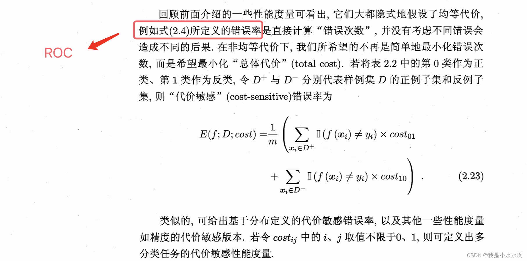
传统的分类算法通常假设所有的错误分类代价是相同的，但在实际应用中，这种情况并不常见。代价敏感错误率的目标是通过考虑不同类别的错误分类代价，使得模型在测试阶段能够最小化总体代价。

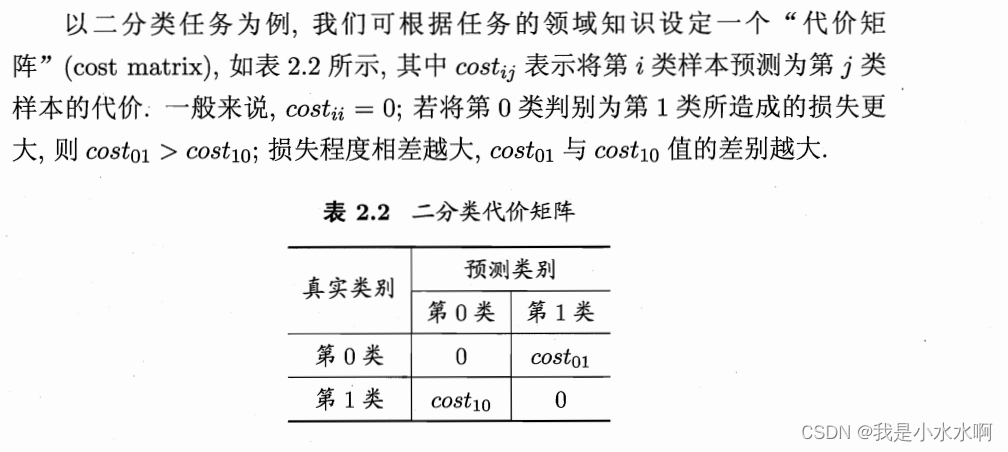
在代价敏感错误率中，通常会引入代价矩阵（cost matrix）来描述不同类别之间的代价关系。代价矩阵是一个二维矩阵，其中的元素c(i, j)表示将真实类别为i的样本误分类为类别j的代价。通过使用代价矩阵，可以在模型训练和评估过程中更好地考虑不同类别的错误分类代价。

在实际应用中，代价敏感错误率通常用于处理那些不同类别错误分类代价差异较大的问题，例如欺诈检测、医学诊断等领域。在训练分类模型时，引入代价矩阵可以帮助模型更好地适应不同类别的代价，从而提高模型在实际应用中的性能。

实现

from sklearn.datasets import load_iris
from sklearn.model_selection import train_test_split
from sklearn.metrics import confusion_matrix
from skmultilearn.problem_transform import ClassifierChain
from sklearn.base import BaseEstimator, ClassifierMixin
from sklearn.ensemble import RandomForestClassifier
import numpy as np

class CostSensitiveClassifier(BaseEstimator, ClassifierMixin):
    def __init__(self, base_estimator=None, cost_matrix=None):
        self.base_estimator = base_estimator
        self.cost_matrix = cost_matrix

    def fit(self, X, y):
        self.base_estimator.fit(X, y)
        return self

    def predict(self, X):
        return self.base_estimator.predict(X)

    def predict_proba(self, X):
        return self.base_estimator.predict_proba(X)

# 以加载iris数据集为例
iris = load_iris()
X = iris.data
y = iris.target

# 将数据集分成训练集和测试集
X_train, X_test, y_train, y_test = train_test_split(X, y, test_size=0.2, random_state=42)

# 定义成本矩阵
# 首先有三种分类所有这个矩阵就是3x3,可以看上面表2.2.的代价矩阵就可以理解了
cost_matrix = np.array([[0, 100, 0],
                        [0, 0, 1000],
                        [0, 0, 0]])

# 使用RandomForestClassifier创建成本敏感分类器作为基本估计器
cost_sensitive_classifier = CostSensitiveClassifier(base_estimator=RandomForestClassifier(random_state=42), cost_matrix=cost_matrix)

# Fit the model
cost_sensitive_classifier.fit(X_train, y_train)

# Make predictions
predictions = cost_sensitive_classifier.predict(X_test)

# Evaluate the model using confusion matrix
conf_matrix = confusion_matrix(y_test, predictions)
print("Confusion Matrix:")
print(conf_matrix)

代价曲线

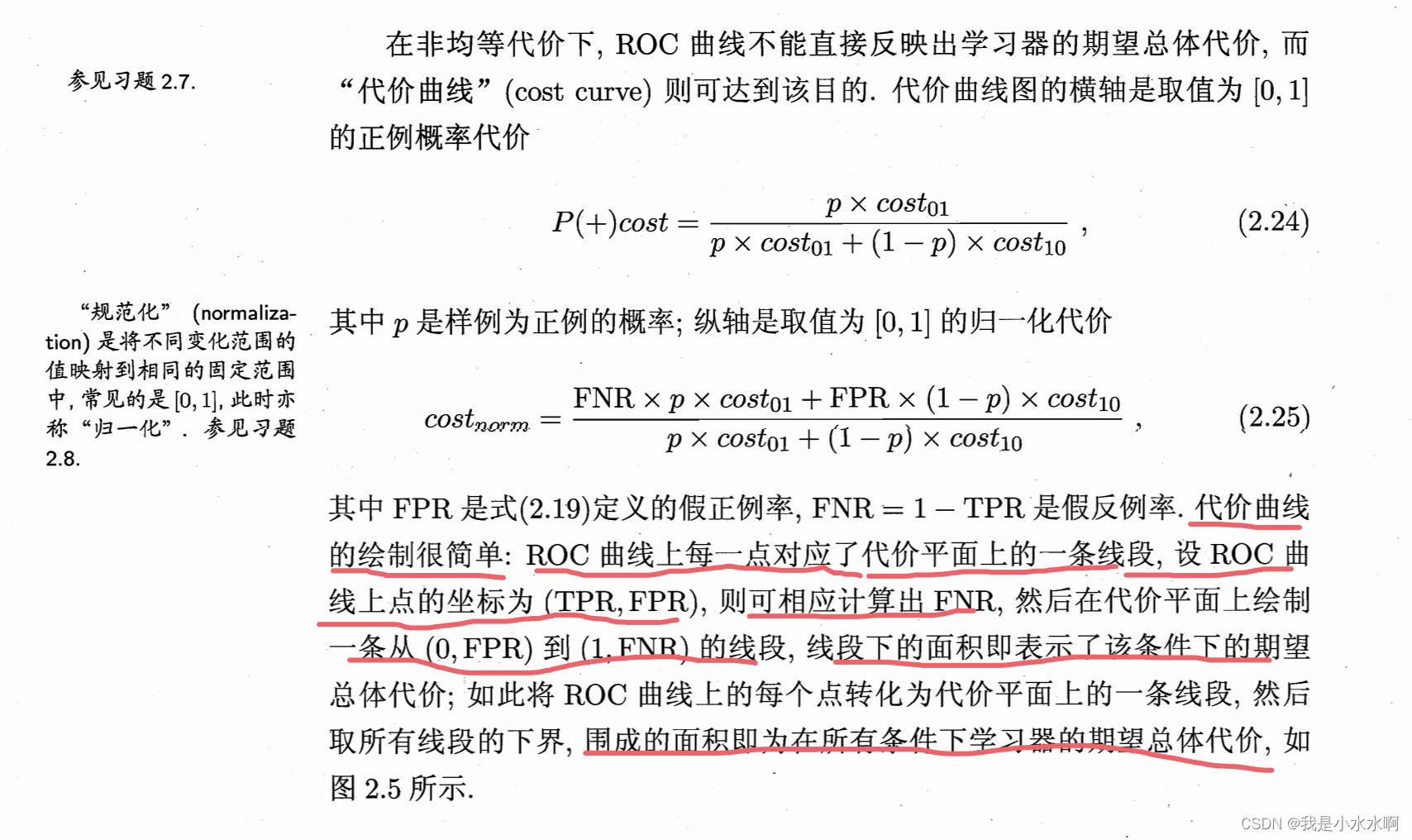
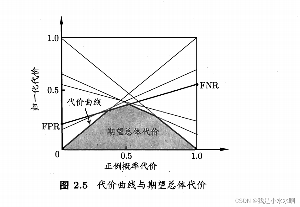
代价曲线（Cost Curve）是一个用于评估代价敏感学习算法性能的工具。在许多实际问题中，不同类别的错误分类可能导致不同的代价。例如，在医疗诊断中，将一个健康患者误诊为患病可能会导致不同于将一个患病患者误诊为健康的代价。代价曲线帮助我们在考虑不同错误分类代价的情况下，选择一个适当的分类阈值。

代价曲线的意义和应用包括以下几点：

1. 选择最优分类阈值： 代价曲线可以帮助你选择一个最适合的分类阈值，使得在考虑不同类别错误分类代价的情况下，总代价最小化。通过观察代价曲线，你可以选择使得总代价最小的分类阈值，从而在实际应用中取得更好的性能。

2. 模型选择和比较： 代价曲线可以用于比较不同模型在代价敏感情况下的性能。通过比较不同模型在代价曲线上的表现，你可以选择最适合你问题的模型。

3. 业务决策支持： 在许多业务场景中，不同类型的错误可能具有不同的后果。例如，在信用卡欺诈检测中，将一个正常交易误判为欺诈交易的代价可能比将一个欺诈交易误判为正常交易的代价大得多。代价曲线可以帮助业务决策者理解模型的性能，并根据业务需求调整模型的阈值。

绘制代价曲线的步骤通常包括以下几个部分：

1. 定义代价矩阵： 首先，你需要明确定义每种错误分类的代价。代价矩阵（cost matrix）是一个二维矩阵，其中的每个元素表示将真实类别i的样本错误地分类为类别j的代价。这个矩阵应该根据你的问题领域和需求来定义。

2. 模型预测概率： 使用你的分类模型（比如随机森林、逻辑回归等）对测试数据集进行预测，并获取每个样本属于各个类别的概率。

3. 计算总代价： 对于每个可能的分类阈值，使用代价矩阵和模型的预测概率计算出混淆矩阵（confusion matrix），然后根据代价矩阵计算总代价。

4. 绘制代价曲线： 将不同分类阈值下的总代价绘制成图表，横轴表示阈值，纵轴表示总代价。通过观察代价曲线，你可以选择使得总代价最小的分类阈值。

以下是在Python中绘制代价曲线的基本步骤示例：

import numpy as np
import matplotlib.pyplot as plt
from sklearn.metrics import confusion_matrix

# 1. 定义代价矩阵
cost_matrix = np.array([[0, 1, 1],
                        [10, 0, 5],
                        [5, 5, 0]])

# 2. 模型预测概率
# 这里假设你已经有了模型的预测概率，存储在变量 predicted_probs 中

# 3. 计算总代价
thresholds = np.linspace(0, 1, 100)
total_costs = []

for threshold in thresholds:
    y_pred_thresholded = np.argmax(predicted_probs, axis=1)
    y_pred_thresholded = np.where(predicted_probs.max(axis=1) > threshold, y_pred_thresholded, -1)
    conf_matrix = confusion_matrix(true_labels, y_pred_thresholded, labels=[0, 1, 2])
    total_cost = np.sum(conf_matrix * cost_matrix)  # 计算总代价
    total_costs.append(total_cost)

# 4. 绘制代价曲线
plt.figure(figsize=(8, 6))
plt.plot(thresholds, total_costs, marker='o', linestyle='-', color='b')
plt.xlabel('Threshold')
plt.ylabel('Total Cost')
plt.title('Cost Curve')
plt.grid(True)
plt.show()

请确保 predicted_probs 包含模型的预测概率，true_labels 包含测试数据的真实类别。这个示例代码中，total_costs 中存储了不同阈值下的总代价，将其绘制成曲线，你就得到了代价曲线。希望这个例子能帮到你理解代价曲线的绘制过程。

例子

import numpy as np
import matplotlib.pyplot as plt
from sklearn.datasets import load_iris
from sklearn.model_selection import train_test_split
from sklearn.ensemble import RandomForestClassifier
from sklearn.metrics import confusion_matrix

# 加载数据 这个类别是有三种
iris = load_iris()
X = iris.data
y = iris.target

# 假设一个代价矩阵，其中假阳性代价为1，类1的假阴性代价为10，类2的假阴性代价为5
cost_matrix = np.array([[0, 1, 1],
                        [10, 0, 5],
                        [5, 5, 0]])

# 将数据集分成训练集和测试集
X_train, X_test, y_train, y_test = train_test_split(X, y, test_size=0.2, random_state=42)

# 训练一个随机森林分类器
rf_classifier = RandomForestClassifier(random_state=42)
rf_classifier.fit(X_train, y_train)

# 作出预测
"""
三个类别（类别0、类别1、类别2），rf_classifier.predict_proba(X_test) 的输出
可能是一个形状为 (n_samples, 3) 的数组，其中 n_samples 
是测试样本的数量。这个数组的每一行表示一个测试样本，每一列的值表示该样本属于对应类别的概率。
"""
y_pred_probs = rf_classifier.predict_proba(X_test)


# 计算每个阈值的总成本
thresholds = np.linspace(0, 1, 100)
total_costs = []

for threshold in thresholds:
    y_pred_thresholded = np.argmax(y_pred_probs, axis=1)
    y_pred_thresholded = np.where(y_pred_probs.max(axis=1) > threshold, y_pred_thresholded, -1)
    conf_matrix = confusion_matrix(y_test, y_pred_thresholded, labels=[0, 1, 2])
    total_cost = np.sum(conf_matrix * cost_matrix)  # 使用给定的成本矩阵计算总成本
    total_costs.append(total_cost)

# Plot the cost curve
plt.figure(figsize=(8, 6))
plt.plot(thresholds, total_costs, marker='o', linestyle='-', color='b')
plt.xlabel('Threshold')
plt.ylabel('Total Cost')
plt.title('Cost Curve')
plt.grid(True)
plt.show()


print(y_pred_probs)