Transformer再出发

这篇文章关于transformer的介绍及实现可谓是非常详细、深刻，之前转载学习过一篇过于transformer的文章，那篇相对来说是一个从宏观逐步到微观组成的，也是非常的经典。推荐先阅读那一篇，再来细细品味这一篇，将会深刻许多。

transformer确实是应用非常广泛，而且达到了目前最优的性能，所以不得不拿过来一遍一遍的品味。本篇文章以转载分享为主，个人理解为辅。

全文如下：

Google 2017年的论文 Attention is all you need 阐释了什么叫做大道至简！该论文提出了Transformer模型，完全基于Attention mechanism，抛弃了传统的RNN和CNN。

我们根据论文的结构图，一步一步使用 PyTorch 实现这个Transformer模型。

Transformer架构

首先看一下transformer的结构图：

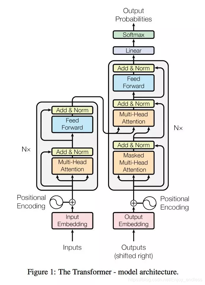
解释一下这个结构图。首先，Transformer模型也是使用经典的encoer-decoder架构，由encoder和decoder两部分组成。

上图的左半边用Nx框出来的，就是我们的encoder的一层。encoder一共有6层这样的结构。

上图的右半边用Nx框出来的，就是我们的decoder的一层。decoder一共有6层这样的结构。

输入序列经过word embedding和positional encoding相加后，输入到encoder。

输出序列经过word embedding和positional encoding相加后，输入到decoder。
最后，decoder输出的结果，经过一个线性层，然后计算softmax。

word embedding和positional encoding我后面会解释。我们首先详细地分析一下encoder和decoder的每一层是怎么样的。

Encoder

encoder由6层相同的层组成，每一层分别由两部分组成：

第一部分是一个multi-head self-attention mechanism
第二部分是一个position-wise feed-forward network，是一个全连接层

两个部分，都有一个残差连接(residual connection)，然后接着一个Layer Normalization。

如果你是一个新手，你可能会问：

multi-head self-attention 是什么呢？
参差结构是什么呢？
Layer Normalization又是什么？

这些问题我们在后面会一一解答。

Decoder

和encoder类似，decoder由6个相同的层组成，每一个层包括以下3个部分：

第一个部分是multi-head self-attention mechanism
第二部分是multi-head context-attention mechanism
第三部分是一个position-wise feed-forward network

还是和encoder类似，上面三个部分的每一个部分，都有一个残差连接，后接一个Layer Normalization。

但是，decoder出现了一个新的东西multi-head context-attention mechanism。这个东西其实也不复杂，理解了multi-head self-attention你就可以理解multi-head context-attention。这个我们后面会讲解。

Attention机制
在讲清楚各种attention之前，我们得先把attention机制说清楚。

通俗来说，attention是指，对于某个时刻的输出y，它在输入x上各个部分的注意力。这个注意力实际上可以理解为权重。

attention机制也可以分成很多种。Attention? Attention! 一问有一张比较全面的表格：

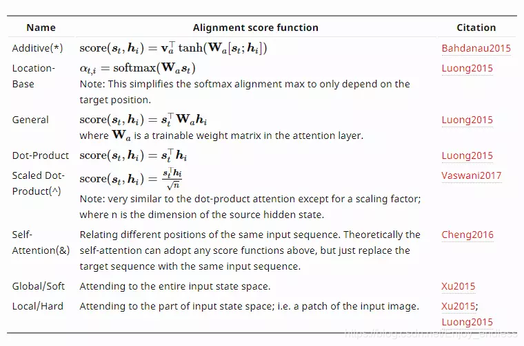
Figure 2. a summary table of several popular attention mechanisms.

上面第一种additive attention你可能听过。以前我们的seq2seq模型里面，使用attention机制，这种**加性注意力(additive attention)**用的很多。Google的项目 tensorflow/nmt 里面使用的attention就是这种。

为什么这种attention叫做additive attention呢？很简单，对于输入序列隐状态和输出序列的隐状态，它的处理方式很简单，直接合并，变成【s;h】

但是我们的transformer模型使用的不是这种attention机制，使用的是另一种，叫做乘性注意力(multiplicative attention)。

那么这种乘性注意力机制是怎么样的呢？从上表中的公式也可以看出来：两个隐状态进行点积！

Self-attention是什么？

到这里就可以解释什么是self-attention了。

上面我们说attention机制的时候，都会说到两个隐状态，分别是hi和st，前者是输入序列第i个位置产生的隐状态，后者是输出序列在第t个位置产生的隐状态。

所谓self-attention实际上就是，输出序列就是输入序列！因此，计算自己的attention得分，就叫做self-attention！（对于自身句子的每一个词的权重关注，即这个词由其这个句子的其他词所组成）

Context-attention是什么？

知道了self-attention，那你肯定猜到了context-attention是什么了：它是encoder和decoder之间的attention！所以，你也可以称之为encoder-decoder attention!(是两个不同句子间的权重表示，或者说是两种不同的句子表示形式之间的权重表示)

context-attention一词并不是本人原创，有些文章或者代码会这样描述，我觉得挺形象的，所以在此沿用这个称呼。其他文章可能会有其他名称，但是不要紧，我们抓住了重点即可，那就是两个不同序列之间的attention，与self-attention相区别。

不管是self-attention还是context-attention，它们计算attention分数的时候，可以选择很多方式，比如上面表中提到的：
additive attention
local-base
general
dot-product
scaled dot-product

那么我们的Transformer模型，采用的是哪种呢？答案是：scaled dot-product attention。

Scaled dot-product attention是什么？
论文Attention is all you need里面对于attention机制的描述是这样的：

An attention function can be described as a query and a set of key-value pairs to an output, where the query, keys, values, and output are all vectors. The output is computed as a weighted sum of the values, where the weight assigned to each value is computed by a compatibility of the query with the corresponding key.
查询q以不同概率对应不同索引k，根据不同k权重(概率)加和对应v来表示输出

这句话描述得很清楚了。翻译过来就是：通过确定Q和K之间的相似程度来选择V！
用公式来描述更加清晰：

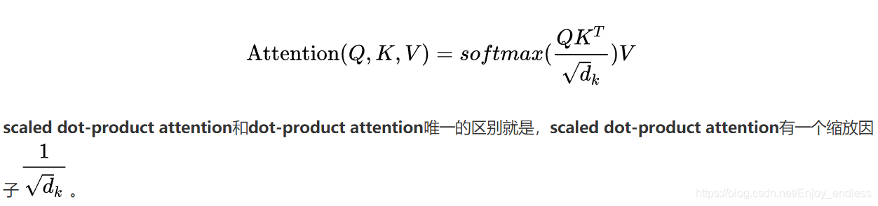
上面公式中的dk表示的是K的维度，在论文里面，默认是64。

那么为什么需要加上这个缩放因子呢？论文里给出了解释：对于很大的时候，点积得到的结果维度很大，使得结果处于softmax函数梯度很小的区域。

我们知道，梯度很小的情况，这对反向传播不利。为了克服这个负面影响，除以一个缩放因子，可以一定程度上减缓这种情况。

论文也提供了一张很清晰的结构图，供大家参考：

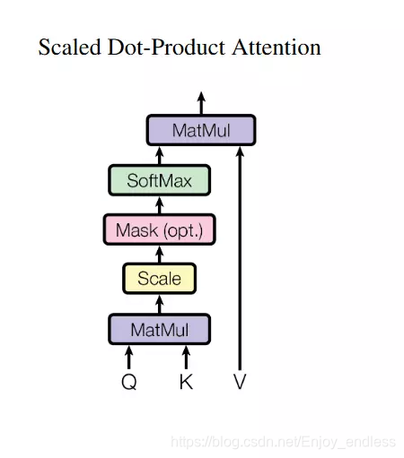
Figure 3. Scaled dot-product attention architecture.

首先说明一下我们的K、Q、V是什么：

##在encoder的self-attention中，Q、K、V都来自同一个地方（相等），他们是上一层encoder的输出。对于第一层encoder，它们就是word embedding和positional encoding相加得到的输入。
##在decoder的self-attention中，Q、K、V都来自于同一个地方（相等），它们是上一层decoder的输出。对于第一层decoder，它们就是word embedding和positional encoding相加得到的输入。但是对于decoder，我们不希望它能获得下一个time step（即将来的信息），因此我们需要进行sequence masking。
##在encoder-decoder attention中，Q来自于decoder的上一层的输出，K和V来自于encoder的输出，K和V是一样的。
##Q、K、V三者的维度一样，即dq=dk=dv 。

上面scaled dot-product attention和decoder的self-attention都出现了masking这样一个东西。那么这个mask到底是什么呢？这两处的mask操作是一样的吗？这个问题在后面会有详细解释。

Scaled dot-product attention的实现

咱们先把scaled dot-product attention实现了吧。代码如下：

import torch
import torch.nn as nn

class ScaledDotProductAttention(nn.Module):
    """Scaled dot-product attention mechanism."""

    def __init__(self, attention_dropout=0.0):
        super(ScaledDotProductAttention, self).__init__()
        self.dropout = nn.Dropout(attention_dropout)
        self.softmax = nn.Softmax(dim=2)

    def forward(self, q, k, v, scale=None, attn_mask=None):
        """前向传播.

        Args:
        	q: Queries张量，形状为[B, L_q, D_q]
        	k: Keys张量，形状为[B, L_k, D_k]
        	v: Values张量，形状为[B, L_v, D_v]，一般来说就是k
        	scale: 缩放因子，一个浮点标量
        	attn_mask: Masking张量，形状为[B, L_q, L_k]

        Returns:
        	上下文张量和attetention张量
        """
        attention = torch.bmm(q, k.transpose(1, 2))
        if scale:
        	attention = attention * scale
        if attn_mask:
        	# 给需要mask的地方设置一个负无穷
        	attention = attention.masked_fill_(attn_mask, -np.inf)
		# 计算softmax
        attention = self.softmax(attention)
		# 添加dropout
        attention = self.dropout(attention)
		# 和V做点积
        context = torch.bmm(attention, v)
        return context, attention

Multi-head attention又是什么呢？

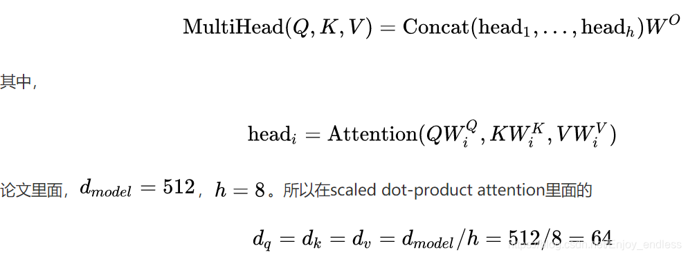
理解了Scaled dot-product attention，Multi-head attention也很简单了。论文提到，他们发现将Q、K、V通过一个线性映射之后，分成h 份，对每一份进行scaled dot-product attention效果更好。然后，把各个部分的结果合并起来，再次经过线性映射，得到最终的输出。这就是所谓的multi-head attention。上面的超参数 就是heads数量。论文默认是8。

下面是multi-head attention的结构图：

Figure 4: Multi-head attention architecture.

值得注意的是，上面所说的分成 h 份是在 dk、dq、dv 维度上面进行切分的。因此，进入到scaled dot-product attention的 dk实际上等于未进入之前的 Dk/h。

Multi-head attention允许模型加入不同位置的表示子空间的信息。

Multi-head attention的公式如下：

Multi-head attention的实现

相信大家已经理清楚了multi-head attention，那么我们来实现它吧。代码如下：

import torch
import torch.nn as nn

class MultiHeadAttention(nn.Module):

    def __init__(self, model_dim=512, num_heads=8, dropout=0.0):
        super(MultiHeadAttention, self).__init__()

        self.dim_per_head = model_dim // num_heads
        self.num_heads = num_heads
        self.linear_k = nn.Linear(model_dim, self.dim_per_head * num_heads)
        self.linear_v = nn.Linear(model_dim, self.dim_per_head * num_heads)
        self.linear_q = nn.Linear(model_dim, self.dim_per_head * num_heads)

        self.dot_product_attention = ScaledDotProductAttention(dropout)
        self.linear_final = nn.Linear(model_dim, model_dim)
        self.dropout = nn.Dropout(dropout)
		# multi-head attention之后需要做layer norm
        self.layer_norm = nn.LayerNorm(model_dim)

    def forward(self, key, value, query, attn_mask=None):
		# 残差连接
        residual = query

        dim_per_head = self.dim_per_head
        num_heads = self.num_heads
        batch_size = key.size(0)

        # linear projection
        key = self.linear_k(key)
        value = self.linear_v(value)
        query = self.linear_q(query)

        # split by heads
        key = key.view(batch_size * num_heads, -1, dim_per_head)
        value = value.view(batch_size * num_heads, -1, dim_per_head)
        query = query.view(batch_size * num_heads, -1, dim_per_head)

        if attn_mask:
            attn_mask = attn_mask.repeat(num_heads, 1, 1)
        # scaled dot product attention
        scale = (key.size(-1) ) ** -0.5
        context, attention = self.dot_product_attention(
          query, key, value, scale, attn_mask)

        # concat heads
        context = context.view(batch_size, -1, dim_per_head * num_heads)

        # final linear projection
        output = self.linear_final(context)

        # dropout
        output = self.dropout(output)

        # add residual and norm layer
        output = self.layer_norm(residual + output)

        return output, attention

上面的代码终于出现了Residual connection和Layer normalization。我们现在来解释它们。

Residual connection是什么？

残差连接其实很简单！给你看一张示意图你就明白了：

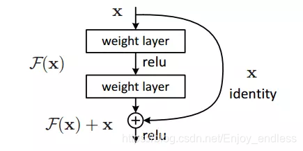
Figure 5. Residual connection.

假设网络中某个层对输入x作用后的输出是F(x)，那么增加residual connection之后，就变成了：
F(x)+x

这个**+x操作就是一个shortcut**。

那么残差结构有什么好处呢？显而易见：因为增加了一项，那么该层网络对x求偏导的时候，多了一个常数项！所以在反向传播过程中，梯度连乘，也不会造成梯度消失！

所以，代码实现residual connection很非常简单：

def residual(sublayer_fn,x):
	return sublayer_fn(x)+x

文章开始的transformer架构图中的Add & Norm中的Add也就是指的这个shortcut。

至此，residual connection的问题理清楚了。更多关于残差网络的介绍可以看文末的参考文献。

Layer normalization是什么？

GRADIENTS, BATCH NORMALIZATION AND LAYER NORMALIZATION一文对normalization有很好的解释：

Normalization有很多种，但是它们都有一个共同的目的，那就是把输入转化成均值为0方差为1的数据。我们在把数据送入激活函数之前进行normalization（归一化），因为我们不希望输入数据落在激活函数的饱和区。

说到normalization，那就肯定得提到Batch Normalization。BN在CNN等地方用得很多。

BN的主要思想就是：在每一层的每一批数据上进行归一化。

我们可能会对输入数据进行归一化，但是经过该网络层的作用后，我们的的数据已经不再是归一化的了。随着这种情况的发展，数据的偏差越来越大，我的反向传播需要考虑到这些大的偏差，这就迫使我们只能使用较小的学习率来防止梯度消失或者梯度爆炸。

BN的具体做法就是对每一小批数据，在批这个方向上做归一化。如下图所示：

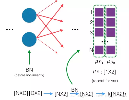
Figure 6. Batch normalization example.(From theneuralperspective.com)

可以看到，右半边求均值是沿着数据批量N的方向进行的！

Batch normalization的计算公式如下：

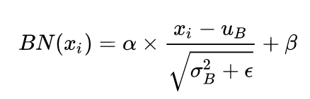
具体的实现可以查看上图的链接文章。

说完Batch normalization，就该说说咱们今天的主角Layer normalization。

那么什么是Layer normalization呢？:它也是归一化数据的一种方式，不过LN是在每一个样本上计算均值和方差，而不是BN那种在批方向计算均值和方差！（一个样本的在多层上的N，而不是一层上的多个样本N）
下面是LN的示意图：

Figure 7. Layer normalization example.

和上面的BN示意图一比较就可以看出二者的区别啦！

下面看一下LN的公式，也BN十分相似：

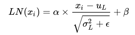
Layer normalization的实现

上述两个参数\alpha和\beta都是可学习参数。下面我们自己来实现Layer normalization(PyTorch已经实现啦！)。代码如下：

import torch
import torch.nn as nn


class LayerNorm(nn.Module):
    """实现LayerNorm。其实PyTorch已经实现啦，见nn.LayerNorm。"""

    def __init__(self, features, epsilon=1e-6):
        """Init.

        Args:
            features: 就是模型的维度。论文默认512
            epsilon: 一个很小的数，防止数值计算的除0错误
        """
        super(LayerNorm, self).__init__()
        # alpha
        self.gamma = nn.Parameter(torch.ones(features))
        # beta
        self.beta = nn.Parameter(torch.zeros(features))
        self.epsilon = epsilon

    def forward(self, x):
        """前向传播.

        Args:
            x: 输入序列张量，形状为[B, L, D]
        """
        # 根据公式进行归一化
        # 在X的最后一个维度求均值，最后一个维度就是模型的维度
        mean = x.mean(-1, keepdim=True)
        # 在X的最后一个维度求方差，最后一个维度就是模型的维度
        std = x.std(-1, keepdim=True)
        return self.gamma * (x - mean) / (std + self.epsilon) + self.beta

顺便提一句，Layer normalization多用于RNN这种结构。

Mask是什么？

现在终于轮到讲解mask了!mask顾名思义就是掩码，在我们这里的意思大概就是对某些值进行掩盖，使其不产生效果。

需要说明的是，我们的Transformer模型里面涉及两种mask。分别是padding mask和sequence mask。其中后者我们已经在decoder的self-attention里面见过啦！

其中，padding mask在所有的scaled dot-product attention里面都需要用到，而sequence mask只有在decoder的self-attention里面用到。
所以，我们之前Scaled Dot Product Attention的forward方法里面的参数attn_mask在不同的地方会有不同的含义。这一点我们会在后面说明。

Padding mask

什么是padding mask呢？回想一下，我们的每个批次输入序列长度是不一样的！也就是说，我们要对输入序列进行对齐！具体来说，就是给在较短的序列后面填充0。因为这些填充的位置，其实是没什么意义的，所以我们的attention机制不应该把注意力放在这些位置上，所以我们需要进行一些处理。

具体的做法是，把这些位置的值加上一个非常大的负数(可以是负无穷)，这样的话，经过softmax，这些位置的概率就会接近0！

而我们的padding mask实际上是一个张量，每个值都是一个Boolen，值为False的地方就是我们要进行处理的地方。
下面是实现：

def padding_mask(seq_k, seq_q):
	# seq_k和seq_q的形状都是[B,L]
    len_q = seq_q.size(1)
    # `PAD` is 0
    pad_mask = seq_k.eq(0)
    pad_mask = pad_mask.unsqueeze(1).expand(-1, len_q, -1)  # shape [B, L_q, L_k]
    return pad_mask

Sequence mask

文章前面也提到，sequence mask是为了使得decoder不能看见未来的信息。也就是对于一个序列，在time_step为t的时刻，我们的解码输出应该只能依赖于t时刻之前的输出，而不能依赖t之后的输出。因此我们需要想一个办法，把t之后的信息给隐藏起来。

那么具体怎么做呢？也很简单：产生一个上三角矩阵，上三角的值全为1，下三角的值权威0，对角线也是0。把这个矩阵作用在每一个序列上，就可以达到我们的目的啦。
具体的代码实现如下：

def sequence_mask(seq):
    batch_size, seq_len = seq.size()
    mask = torch.triu(torch.ones((seq_len, seq_len), dtype=torch.uint8),
                    diagonal=1)
    mask = mask.unsqueeze(0).expand(batch_size, -1, -1)  # [B, L, L]
    return mask

哈佛大学的文章The Annotated Transformer有一张效果图:

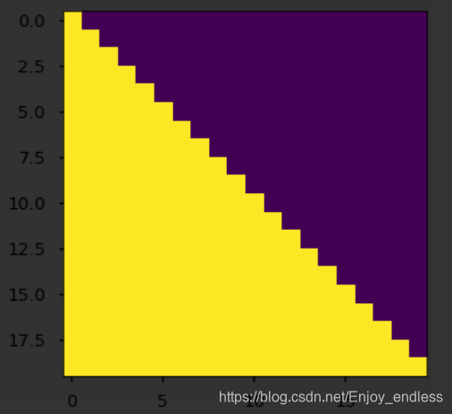
Figure 8. Sequence mask.

值得注意的是，本来mask只需要二维的矩阵即可，但是考虑到我们的输入序列都是批量的，所以我们要把原本二维的矩阵扩张成3维的张量。上面的代码可以看出，我们已经进行了处理。

回到本小结开始的问题，attn_mask参数有几种情况？分别是什么意思？

##对于decoder的self-attention，里面使用到的scaled dot-product attention，同时需要padding mask和sequence mask作为attn_mask，具体实现就是两个mask相加作为attn_mask。
##其他情况，attn_mask一律等于padding mask。

至此，mask相关的问题解决了。

Positional encoding是什么？

好了，终于要解释位置编码了，那就是文字开始的结构图提到的Positional encoding。

就目前而言，我们的Transformer架构似乎少了点什么东西。没错，就是它对序列的顺序没有约束！我们知道序列的顺序是一个很重要的信息，如果缺失了这个信息，可能我们的结果就是：所有词语都对了，但是无法组成有意义的语句！

为了解决这个问题。论文提出了Positional encoding。这是啥？一句话概括就是：对序列中的词语出现的位置进行编码！如果对位置进行编码，那么我们的模型就可以捕捉顺序信息！

那么具体怎么做呢？论文的实现很有意思，使用正余弦函数。公式如下：

其中，pos是指词语在序列中的位置。可以看出，在偶数位置，使用正弦编码，在奇数位置，使用余弦编码。

上面公式中的是模型的维度，论文默认是512。

这个编码公式的意思就是：给定词语的位置pos，我们可以把它编码成d_model维的向量！也就是说，位置编码的每一个维度对应正弦曲线，波长构成了2pai到100002*pai的等比序列。

上面的位置编码是绝对位置编码。但是词语的相对位置也非常重要。这就是论文为什么要使用三角函数的原因！

正弦函数能够表达相对位置信息。，主要数学依据是以下两个公式：

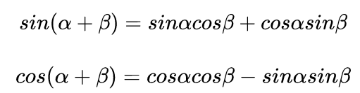
上面的公式说明，对于词汇之间的位置偏移k，PE(pos+k)可以表示成PE(pos)和PE(k)的组合形式，这就是表达相对位置的能力！

以上就是PE的所有秘密。说完了positional encoding，那么我们还有一个与之处于同一地位的word embedding。

Word embedding大家都很熟悉了，它是对序列中的词汇的编码，把每一个词汇编码成d_model维的向量！看到没有，Postional encoding是对词汇的位置编码，word embedding是对词汇本身编码！

所以，我更喜欢positional encoding的另外一个名字Positional embedding！

Positional encoding的实现

PE的实现也不难，按照论文的公式即可。代码如下：

class PositionalEncoding(nn.Module):
    
    def __init__(self, d_model, max_seq_len):
        """初始化。
        
        Args:
            d_model: 一个标量。模型的维度，论文默认是512
            max_seq_len: 一个标量。文本序列的最大长度
        """
        super(PositionalEncoding, self).__init__()
        
        # 根据论文给的公式，构造出PE矩阵
        position_encoding = np.array([
          [pos / np.pow(10000, 2.0 * (j // 2) / d_model) for j in range(d_model)]
          for pos in range(max_seq_len)])
        # 偶数列使用sin，奇数列使用cos
        position_encoding[:, 0::2] = np.sin(position_encoding[:, 0::2])
        position_encoding[:, 1::2] = np.cos(position_encoding[:, 1::2])

        # 在PE矩阵的第一行，加上一行全是0的向量，代表这`PAD`的positional encoding
        # 在word embedding中也经常会加上`UNK`，代表位置单词的word embedding，两者十分类似
        # 那么为什么需要这个额外的PAD的编码呢？很简单，因为文本序列的长度不一，我们需要对齐，
        # 短的序列我们使用0在结尾补全，我们也需要这些补全位置的编码，也就是`PAD`对应的位置编码
        pad_row = torch.zeros([1, d_model])
        position_encoding = torch.cat((pad_row, position_encoding))
        
        # 嵌入操作，+1是因为增加了`PAD`这个补全位置的编码，
        # Word embedding中如果词典增加`UNK`，我们也需要+1。看吧，两者十分相似
        self.position_encoding = nn.Embedding(max_seq_len + 1, d_model)
        self.position_encoding.weight = nn.Parameter(position_encoding,
                                                     requires_grad=False)
    def forward(self, input_len):
        """神经网络的前向传播。

        Args:
          input_len: 一个张量，形状为[BATCH_SIZE, 1]。每一个张量的值代表这一批文本序列中对应的长度。

        Returns:
          返回这一批序列的位置编码，进行了对齐。
        """
        
        # 找出这一批序列的最大长度
        max_len = torch.max(input_len)
        tensor = torch.cuda.LongTensor if input_len.is_cuda else torch.LongTensor
        # 对每一个序列的位置进行对齐，在原序列位置的后面补上0
        # 这里range从1开始也是因为要避开PAD(0)的位置
        input_pos = tensor(
          [list(range(1, len + 1)) + [0] * (max_len - len) for len in input_len])
        return self.position_encoding(input_pos)

Word embedding的实现

Word embedding应该是老生常谈了，它实际上就是一个二维浮点矩阵，里面的权重是可训练参数，我们只需要把这个矩阵构建出来就完成了word embedding的工作。

所以，具体的实现很简单：

import torch.nn as nn


embedding = nn.Embedding(vocab_size, embedding_size, padding_idx=0)
# 获得输入的词嵌入编码
seq_embedding = seq_embedding(inputs)*np.sqrt(d_model)

上面vocab_size就是词典的大小，embedding_size就是词嵌入的维度大小，论文里面就是等于d_model=512。所以word embedding矩阵就是一个vocab_size*embedding_size的二维张量。

如果你想获取更详细的关于word embedding的信息，可以看我的另外一个文章word2vec的笔记和实现。

Position-wise Feed-Forward network是什么？

这就是一个全连接网络，包含两个线性变换和一个非线性函数（实际上就是ReLU）。公式如下：

这个线性变换在不同的位置都表现地一样，并且在不同的层之间使用不同的参数。
论文提到，这个公式还可以用两个核大小为1的一维卷积来解释，卷积的输入输出都是d_model=512，中间层的维度是dff=2048。

实现如下：

import torch
import torch.nn as nn

class PositionalWiseFeedForward(nn.Module):

    def __init__(self, model_dim=512, ffn_dim=2048, dropout=0.0):
        super(PositionalWiseFeedForward, self).__init__()
        self.w1 = nn.Conv1d(model_dim, ffn_dim, 1)
        self.w2 = nn.Conv1d(model_dim, ffn_dim, 1)
        self.dropout = nn.Dropout(dropout)
        self.layer_norm = nn.LayerNorm(model_dim)

    def forward(self, x):
        output = x.transpose(1, 2)
        output = self.w2(F.relu(self.w1(output)))
        output = self.dropout(output.transpose(1, 2))

        # add residual and norm layer
        output = self.layer_norm(x + output)
        return output

Transformer的实现

至此，所有的细节都已经解释完了。现在来完成我们Transformer模型的代码。

首先，我们需要实现6层的encoder和decoder。

encoder代码实现如下：

import torch
import torch.nn as nn


class EncoderLayer(nn.Module):
	"""Encoder的一层。"""

    def __init__(self, model_dim=512, num_heads=8, ffn_dim=2018, dropout=0.0):
        super(EncoderLayer, self).__init__()

        self.attention = MultiHeadAttention(model_dim, num_heads, dropout)
        self.feed_forward = PositionalWiseFeedForward(model_dim, ffn_dim, dropout)

    def forward(self, inputs, attn_mask=None):

        # self attention
        context, attention = self.attention(inputs, inputs, inputs, padding_mask)

        # feed forward network
        output = self.feed_forward(context)

        return output, attention


class Encoder(nn.Module):
	"""多层EncoderLayer组成Encoder。"""

    def __init__(self,
               vocab_size,
               max_seq_len,
               num_layers=6,
               model_dim=512,
               num_heads=8,
               ffn_dim=2048,
               dropout=0.0):
        super(Encoder, self).__init__()

        self.encoder_layers = nn.ModuleList(
          [EncoderLayer(model_dim, num_heads, ffn_dim, dropout) for _ in
           range(num_layers)])

        self.seq_embedding = nn.Embedding(vocab_size + 1, model_dim, padding_idx=0)
        self.pos_embedding = PositionalEncoding(model_dim, max_seq_len)

    def forward(self, inputs, inputs_len):
        output = self.seq_embedding(inputs)
        output += self.pos_embedding(inputs_len)

        self_attention_mask = padding_mask(inputs, inputs)

        attentions = []
        for encoder in self.encoder_layers:
            output, attention = encoder(output, self_attention_mask)
            attentions.append(attention)

        return output, attentions

通过文章前面的分析，代码不需要更多解释了。同样的，我们的decoder代码如下：

import torch
import torch.nn as nn


class DecoderLayer(nn.Module):

    def __init__(self, model_dim, num_heads=8, ffn_dim=2048, dropout=0.0):
        super(DecoderLayer, self).__init__()

        self.attention = MultiHeadAttention(model_dim, num_heads, dropout)
        self.feed_forward = PositionalWiseFeedForward(model_dim, ffn_dim, dropout)

    def forward(self,
              dec_inputs,
              enc_outputs,
              self_attn_mask=None,
              context_attn_mask=None):
        # self attention, all inputs are decoder inputs
        dec_output, self_attention = self.attention(
          dec_inputs, dec_inputs, dec_inputs, self_attn_mask)

        # context attention
        # query is decoder's outputs, key and value are encoder's inputs
        dec_output, context_attention = self.attention(
          enc_outputs, enc_outputs, dec_output, context_attn_mask)

        # decoder's output, or context
        dec_output = self.feed_forward(dec_output)

        return dec_output, self_attention, context_attention


class Decoder(nn.Module):

    def __init__(self,
               vocab_size,
               max_seq_len,
               num_layers=6,
               model_dim=512,
               num_heads=8,
               ffn_dim=2048,
               dropout=0.0):
        super(Decoder, self).__init__()

        self.num_layers = num_layers

        self.decoder_layers = nn.ModuleList(
          [DecoderLayer(model_dim, num_heads, ffn_dim, dropout) for _ in
           range(num_layers)])

        self.seq_embedding = nn.Embedding(vocab_size + 1, model_dim, padding_idx=0)
        self.pos_embedding = PositionalEncoding(model_dim, max_seq_len)

    def forward(self, inputs, inputs_len, enc_output, context_attn_mask=None):
        output = self.seq_embedding(inputs)
        output += self.pos_embedding(inputs_len)

        self_attention_padding_mask = padding_mask(inputs, inputs)
        seq_mask = sequence_mask(inputs)
        self_attn_mask = torch.gt((self_attention_padding_mask + seq_mask), 0)

        self_attentions = []
        context_attentions = []
        for decoder in self.decoder_layers:
            output, self_attn, context_attn = decoder(
            output, enc_output, self_attn_mask, context_attn_mask)
            self_attentions.append(self_attn)
            context_attentions.append(context_attn)

        return output, self_attentions, context_attentions

最后，我们把encoder和decoder组成Transformer模型！

代码如下：

import torch
import torch.nn as nn


class Transformer(nn.Module):

    def __init__(self,
               src_vocab_size,
               src_max_len,
               tgt_vocab_size,
               tgt_max_len,
               num_layers=6,
               model_dim=512,
               num_heads=8,
               ffn_dim=2048,
               dropout=0.2):
        super(Transformer, self).__init__()

        self.encoder = Encoder(src_vocab_size, src_max_len, num_layers, model_dim,
                               num_heads, ffn_dim, dropout)
        self.decoder = Decoder(tgt_vocab_size, tgt_max_len, num_layers, model_dim,
                               num_heads, ffn_dim, dropout)

        self.linear = nn.Linear(model_dim, tgt_vocab_size, bias=False)
        self.softmax = nn.Softmax(dim=2)

    def forward(self, src_seq, src_len, tgt_seq, tgt_len):
        context_attn_mask = padding_mask(tgt_seq, src_seq)

        output, enc_self_attn = self.encoder(src_seq, src_len)

        output, dec_self_attn, ctx_attn = self.decoder(
          tgt_seq, tgt_len, output, context_attn_mask)

        output = self.linear(output)
        output = self.softmax(output)

        return output, enc_self_attn, dec_self_attn, ctx_attn

至此，Transformer模型已经实现了！

作者：luozhouyang
链接：https://juejin.im/post/5b9f1af0e51d450e425eb32d
来源：掘金
著作权归作者所有。商业转载请联系作者获得授权，非商业转载请注明出处。