CAFFE 简单使用教程（无安装部分）

最新推荐文章于 2024-05-03 15:15:30 发布

Fate_fjh

最新推荐文章于 2024-05-03 15:15:30 发布

阅读量1.5k

点赞数 1

本文链接：https://blog.csdn.net/Fate_fjh/article/details/52073446

版权

深度学习专栏收录该内容

9 篇文章 16 订阅

订阅专栏

前言

这里是从caffe成功安装开始，包括caffe的python接口，整个过程就是从训练自己图片到使用自己训练好的模型进行图片分类，这里使用的网络是lenet。

1.预处理

caffe提供了一个生成lmdb的.sh脚本，使用脚本之前需要將图片的绝对路径或者相对路径放在一个txt中，分为train.txt与val.txt。这里我训练样本的文件结构，

这里写图片描述

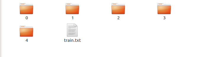
 0,1,2,3,4代表一类图片，例如0的文件夹里面只有bus。 train.txt就是一个需要的训练样本路径，

这里写图片描述
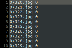
我这里使用的是路径的一部分，当然可以好使用完整的路径，这个后面的create*.sh脚本里面的参数相关。
同理，我们还需要val.txt，val中的数据格式与train.txt一样。这样我们就准备好了train.txt与val.txt。
我们看一下create*.sh脚本，

#!/usr/bin/env sh
# Create the imagenet lmdb inputs
# N.B. set the path to the imagenet train + val data dirs
set -e

EXAMPLE=/home/fung/workspace/lenet_test  #这里的EXAMPLE指的是根目录 
DATA=/home/fung/workspace/lenet_test    #DATA是图片所在位置,这里与EXAMPLE是一样的路径 
TOOLS=/usr/software/caffe/build/tools  #caffe的工具路径

TRAIN_DATA_ROOT=/home/fung/workspace/lenet_test/train/     #训练样本路径
VAL_DATA_ROOT=/home/fung/workspace/lenet_test/test/     #测试样本路径

# Set RESIZE=true to resize the images to 256x256. Leave as false if images have
# already been resized using another tool.
RESIZE=true         #是否需要改变图片大小
if $RESIZE; then
  RESIZE_HEIGHT=150   #图片高度
  RESIZE_WIDTH=150    #图片宽度
else
  RESIZE_HEIGHT=0
  RESIZE_WIDTH=0
fi

if [ ! -d "$TRAIN_DATA_ROOT" ]; then
  echo "Error: TRAIN_DATA_ROOT is not a path to a directory: $TRAIN_DATA_ROOT"
  echo "Set the TRAIN_DATA_ROOT variable in create_imagenet.sh to the path" \
       "where the ImageNet training data is stored."
  exit 1
fi

if [ ! -d "$VAL_DATA_ROOT" ]; then
  echo "Error: VAL_DATA_ROOT is not a path to a directory: $VAL_DATA_ROOT"
  echo "Set the VAL_DATA_ROOT variable in create_imagenet.sh to the path" \
       "where the ImageNet validation data is stored."
  exit 1
fi

echo "Creating train lmdb..."

GLOG_logtostderr=1 $TOOLS/convert_imageset \
    --resize_height=$RESIZE_HEIGHT \
    --resize_width=$RESIZE_WIDTH \
    --shuffle \
    $TRAIN_DATA_ROOT \
    $DATA/train/train.txt \
    $EXAMPLE/lenet_train_lmdb    #输出训练lmdb

echo "Creating val lmdb..."

GLOG_logtostderr=1 $TOOLS/convert_imageset \
    --resize_height=$RESIZE_HEIGHT \
    --resize_width=$RESIZE_WIDTH \
    --shuffle \
    $VAL_DATA_ROOT \
    $DATA/test/val.txt \
    $EXAMPLE/lenet_val_lmdb    #输出测试lmdb

echo "Done."

我建议尽量使用绝对路径，因为相对路径可能会出现一些问题。按照自己的路径设定，这样就可以生成lmdb的文件，有两个文件夹，每个文件夹里面有两个文件。
这里需要强调说明的是：TRAIN_DATA_ROOT与train.txt的路径结合起来是一个图片的完整路径，在设定时不要重复。

有了lmdb之后我们需要一个平均值，caffe有一个mean*.sh求出刚刚得到的lmdb里面数据的平均值。

#!/usr/bin/env sh
# Compute the mean image from the imagenet training lmdb
# N.B. this is available in data/ilsvrc12
EXAMPLE=/home/fung/workspace/lenet_test  #这里的EXAMPLE指的是根目录 
DATA=/home/fung/workspace/lenet_test    #DATA是图片所在位置,这里与EXAMPLE是一样的路径 
TOOLS=/usr/software/caffe/build/tools  #caffe的工具路径

$TOOLS/compute_image_mean $EXAMPLE/lenet_train_lmdb \
  $DATA/lenet_mean.binaryproto
#输出平均值文件
echo "Done."

2.网络的生成

caffe需要一个训练的网络，还需要一个测试的网络，这里给出python的网络例子，

# -*- coding: utf-8 -*-
import caffe
from caffe import layers as L,params as P,to_proto
path='/home/fung/workspace/lenet_test/'                    #保存数据和配置文件的路径
train_lmdb=path+'lenet_train_lmdb'                #训练数据LMDB文件的位置
val_lmdb=path+'lenet_val_lmdb'                    #验证数据LMDB文件的位置
mean_file=path+'lenet_mean.binaryproto'         #均值文件的位置
train_proto=path+'lenet_py/train.prototxt'         #生成的训练配置文件保存的位置
val_proto=path+'lenet_py/val.prototxt'             #生成的验证配置文件保存的位置


#编写一个函数，用于生成网络
def create_net(lmdb,batch_size,include_acc=False):
    #创建第一层：数据层。向上传递两类数据：图片数据和对应的标签
    n = caffe.NetSpec()  #需要加入这个网络层名字的输出才是标准输出
    n.data, n.label = L.Data(source=lmdb, backend=P.Data.LMDB, batch_size=batch_size, ntop=2,
        transform_param=dict(scale=1./255, mirror=True))
    #创建第二屋：卷积层
    n.conv1=L.Convolution(n.data, kernel_size=5, stride=1, num_output=20, weight_filler=dict(type='xavier'), bias_filler=dict(type='constant'))
    n.pool1=L.Pooling(n.conv1, pool=P.Pooling.MAX, kernel_size=2, stride=2)
    n.conv2=L.Convolution(n.pool1, kernel_size=5, stride=1,num_output=50, weight_filler=dict(type='xavier'), bias_filler=dict(type='constant'))
    n.pool2=L.Pooling(n.conv2, pool=P.Pooling.MAX, kernel_size=2, stride=2)
    #创建一个全连接层
    n.ip1=L.InnerProduct(n.pool2, num_output=500, param=[dict(lr_mult=1), dict(lr_mult=2)], weight_filler=dict(type='xavier'), bias_filler=dict(type='constant'))
    #创建激活函数层
    n.relu1=L.ReLU(n.ip1, in_place=True)
    n.ip2=L.InnerProduct(n.ip1, num_output=5, param=[dict(lr_mult=1), dict(lr_mult=2)], weight_filler=dict(type='xavier'), bias_filler=dict(type='constant'))
    #创建一个softmax层
    n.loss = L.SoftmaxWithLoss(n.ip2, n.label)    
    if include_acc:             #在训练阶段，不需要accuracy层，但是在验证阶段，是需要的
        n.acc = L.Accuracy(n.ip2, n.label)
        return n.to_proto()
    else:
        return n.to_proto()

def write_net():
    #将以上的设置写入到prototxt文件
    with open(train_proto, 'w') as f:
        f.write(str(create_net(train_lmdb,batch_size=10)))

    #写入配置文件    
    with open(val_proto, 'w') as f:
        f.write(str(create_net(val_lmdb,batch_size=2, include_acc=True)))

if __name__ == '__main__':
    write_net()

最后生成一个train.prototxt与一个val.prototxt。

这时我们需要一个solver.prototxt，给出python生成的例子

# -*- coding: utf-8 -*-

from caffe.proto import caffe_pb2 
s = caffe_pb2.SolverParameter()

path='/home/fung/workspace/imagenet_test/'  #根目录
solver_file=path+'imagenet_py/solver.prototxt' #输出文件路径

s.train_net = path+'imagenet_py/train.prototxt' #训练网络路径
s.test_net.append(path+'imagenet_py/val.prototxt') #测试网络路径
s.test_interval = 100   #测试迭代间隔
s.test_iter.append(50)  #测试迭代次数
s.max_iter = 10000      #最大迭代次数

s.base_lr = 0.001       #学习速率基准
s.momentum = 0.9        #动量大小
s.weight_decay = 5e-4   #dacay大小
s.lr_policy = 'step'    #学习策略
s.stepsize=10000        #step步长
s.gamma = 0.1     
s.display = 1000        #每隔多少迭代显示结果
s.snapshot = 20000      #每隔多少迭代保存当前快照
s.snapshot_prefix = 'shapshot'
s.type = "SGD"          #随机梯度 
s.solver_mode = caffe_pb2.SolverParameter.GPU  #GPU模式

with open(solver_file, 'w') as f:
    f.write(str(s))

生成的solver.prototxt如下，

train_net: "/home/fung/workspace/imagenet_test/imagenet_py/train.prototxt"
test_net: "/home/fung/workspace/imagenet_test/imagenet_py/val.prototxt"
test_iter: 50
test_interval: 100
base_lr: 0.001
display: 1000
max_iter: 10000
lr_policy: "step"
gamma: 0.1
momentum: 0.9
weight_decay: 0.0005
stepsize: 10000
snapshot: 20000
snapshot_prefix: "shapshot"
solver_mode: GPU
type: "SGD"

到这里，网络就构建完毕。
到caffe根目录，执行（自行更改路径），就开始训练了。

./build/tools/caffe train --solver=models/bvlc_reference_caffenet/solver.prototxt

3.使用训练完的模型进行分类

还是使用一个python来实现，

#coding=utf-8

import caffe
import numpy as np
root='/home/fung/workspace/imagenet_test/'   #根目录
deploy=root + 'imagenet_py/deploy.prototxt'    #deploy文件
caffe_model=root + 'caffe_train/_iter_5000.caffemodel'   #训练好的 caffemodel
img=root+'images.jpeg'    #随机找的一张待测图片
labels_filename = root + 'test/synset_words.txt'  #类别名称文件，将数字标签转换回类别名称

net = caffe.Net(deploy,caffe_model,caffe.TEST)   #加载model和network

#图片预处理设置
transformer = caffe.io.Transformer({'data': net.blobs['data'].data.shape})  #设定图片的shape格式(1,3,28,28)
transformer.set_transpose('data', (2,0,1))    #改变维度的顺序，由原始图片(28,28,3)变为(3,28,28)
#transformer.set_mean('data', np.load(mean_file).mean(1).mean(1))    #减去均值，前面训练模型时没有减均值，这儿就不用
transformer.set_raw_scale('data', 255)    # 缩放到【0，255】之间
transformer.set_channel_swap('data', (2,1,0))   #交换通道，将图片由RGB变为BGR

im=caffe.io.load_image(img)                   #加载图片
net.blobs['data'].data[...] = transformer.preprocess('data',im)      #执行上面设置的图片预处理操作，并将图片载入到blob中

#执行测试
out = net.forward()

labels = np.loadtxt(labels_filename, str, delimiter='\t')   #读取类别名称文件
prob= net.blobs['prob'].data[0].flatten() #取出最后一层（Softmax）属于某个类别的概率值，并打印
print prob
order=prob.argsort()[-1]  #将概率值排序，取出最大值所在的序号 
print 'the class is:',labels[order]   #将该序号转换成对应的类别名称，并打印