Stanford UFLDL教程 Exercise:Sparse Autoencoder

Download Related Reading

• sparseae_reading.pdf
• sparseae_exercise.pdf

Sparse autoencoder implementation

In this problem set, you will implement the sparse autoencoderalgorithm, and show how it discovers that edges are a goodrepresentation for natural images. (Images provided byBruno Olshausen.) The sparse autoencoder algorithm is described inthe lecture notes found on the course website.

In the file sparseae_exercise.zip, we have provided some starter code inMatlab. You should write your code at the places indicatedin the files ("YOUR CODE HERE"). You have to complete the following files:sampleIMAGES.m, sparseAutoencoderCost.m, computeNumericalGradient.m. The starter code in train.m shows how these functions are used.

Specifically, in this exercise you will implement a sparse autoencoder, trained with 8×8 image patches using the L-BFGS optimization algorithm.

A note on the software: The provided .zip file includes a subdirectoryminFunc with 3rd party software implementing L-BFGS, that is licensed under a Creative Commons, Attribute, Non-Commercial license. If you need to use this software for commercial purposes, you can download and use a different function (fminlbfgs) that can serve the samepurpose, but runs ~3x slower for this exercise (and thus is less recommended). You can read more about this in the Fminlbfgs_Details page.

Step 1: Generate training set

The first step is to generate a training set. To get a single training example x, randomly pick one of the 10 images, then randomly sample an 8×8 image patch from the selected image, and convert the image patch (either in row-major order or column-major order; it doesn't matter) into a 64-dimensional vector to get a training example

Complete the code in sampleIMAGES.m. Your code should sample 10000 image patches and concatenate them into a 64×10000 matrix.

To make sure your implementation is working, run the code in "Step 1" of train.m.This should result in a plot of a random sample of 200 patches from the dataset.

Implementational tip: When we run our implemented sampleImages(), it takes under 5 seconds. If your implementationtakes over 30 seconds, it may be because you are accidentally making acopy of an entire 512×512 image each time you're picking a randomimage. By copying a 512×512 image 10000 times, this can make yourimplementation much less efficient. While this doesn't slow down yourcode significantly for this exercise (because we have only 10000examples), when we scale to much larger problems later this quarterwith 10⁶ or more examples, this will significantly slow down yourcode. Please implement sampleIMAGES so that you aren't making acopy of an entire 512×512 image each time you need to cut out an 8x8image patch.

Step 2: Sparse autoencoder objective

Implement code to compute the sparse autoencoder cost function J_sparse(W,b) (Section 3 of the lecture notes)and the corresponding derivatives of J_sparse with respect to the different parameters. Use the sigmoid function for the activation function, . In particular, complete the code in sparseAutoencoderCost.m.

The sparse autoencoder is parameterized by matrices , vectors , .However, for subsequent notational convenience, we will "unroll" all of these parametersinto a very long parameter vector θ with s₁s₂ + s₂s₃ + s₂ + s₃ elements. Thecode for converting between the (W⁽¹⁾,W⁽²⁾,b⁽¹⁾,b⁽²⁾) and the θ parameterization is already provided in the starter code.

Implementational tip: The objective J_sparse(W,b) contains 3 terms, correspondingto the squared error term, the weight decay term, and the sparsity penalty. You're welcometo implement this however you want, but for ease of debugging,you might implement the cost function and derivative computation (backpropagation) only for the squared error term first (this corresponds to setting λ = β = 0), and implement the gradient checking method in the next section to first verify that this code is correct. Then onlyafter you have verified that the objective and derivative calculations corresponding to the squared error term are working, add in code to compute the weight decay and sparsity penalty terms and their corresponding derivatives.

Step 3: Gradient checking

Following Section 2.3 of the lecture notes, implement code for gradient checking. Specifically, complete the code in computeNumericalGradient.m. Please use EPSILON = 10^-4 as described in the lecture notes.

We've also provided code in checkNumericalGradient.m for you to test your code. This code defines a simple quadratic function given by 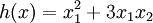, and evaluates it at the point x = (4,10)^T. It allows youto verify that your numerically evaluated gradient is very close to the true (analyticallycomputed) gradient.

After using checkNumericalGradient.m to make sure your implementation is correct, next use computeNumericalGradient.m to make sure that your sparseAutoencoderCost.mis computing derivatives correctly. For details, see Steps 3 in train.m. We stronglyencourage you not to proceed to the next step until you've verified that your derivativecomputations are correct.

Implementational tip: If you are debugging your code, performing gradient checking on smaller models and smaller training sets (e.g., using only 10 training examples and 1-2 hidden units) may speed things up.

Step 4: Train the sparse autoencoder

Now that you have code that computes J_sparse and its derivatives, we're ready to minimize J_sparse with respect to its parameters, and thereby train oursparse autoencoder.

We will use the L-BFGS algorithm. This is provided to you in a function calledminFunc (code provided by Mark Schmidt) included in the starter code. (For the purpose of thisassignment, you only need to call minFunc with the default parameters. You donot need to know how L-BFGS works.) We have already provided code in train.m(Step 4) to call minFunc. The minFunc code assumes that the parametersto be optimized are a long parameter vector; so we will use the "θ" parameterizationrather than the "(W⁽¹⁾,W⁽²⁾,b⁽¹⁾,b⁽²⁾)" parameterization when passing our parametersto it.

Train a sparse autoencoder with 64 input units, 25 hidden units, and 64 output units.In our starter code, we have provided a function for initializing the parameters.We initialize the biases to zero, and the weights to random numbers drawn uniformly from the interval , where n_in is the fan-in(the number of inputs feeding into a node) and n_out is the fan-in (the number ofunits that a node feeds into).

The values we provided for the various parameters (λ,β,ρ, etc.)should work, but feel free to play with different settings of the parameters aswell.

Implementational tip: Once you have your backpropagation implementation correctly computing the derivatives (as verified using gradient checking in Step 3), when you are now using it with L-BFGS to optimize J_sparse(W,b), make sure you're not doing gradient-checking on every step. Backpropagation can be used to compute the derivatives of J_sparse(W,b) fairly efficiently, and if you were additionally computing the gradient numerically on every step, this would slow down your program significantly.

Step 5: Visualization

After training the autoencoder, use display_network.m to visualize the learnedweights. (See train.m, Step 5.) Run "print -djpeg weights.jpg" to savethe visualization to a file "weights.jpg" (which you will submit together withyour code).

Results

To successfully complete this assignment, you should demonstrate your sparseautoencoder algorithm learning a set of edge detectors. For example, thiswas the visualization we obtained:

Our implementation took around 5 minutes to run on a fast computer.In case you end up needing to try out multiple implementations or different parameter values, be sure to budget enough time for debugging and to run the experiments you'll need.

Also, by way of comparison, here are some visualizations from implementationsthat we do not consider successful (either a buggy implementation, or wherethe parameters were poorly tuned):

from： http://ufldl.stanford.edu/wiki/index.php/Exercise:Sparse_Autoencoder