【文献分享】Modelling the species-area提供数据和代码

介绍

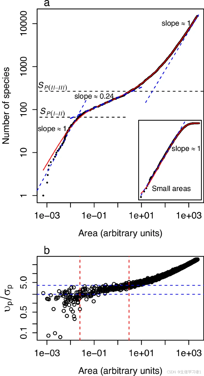
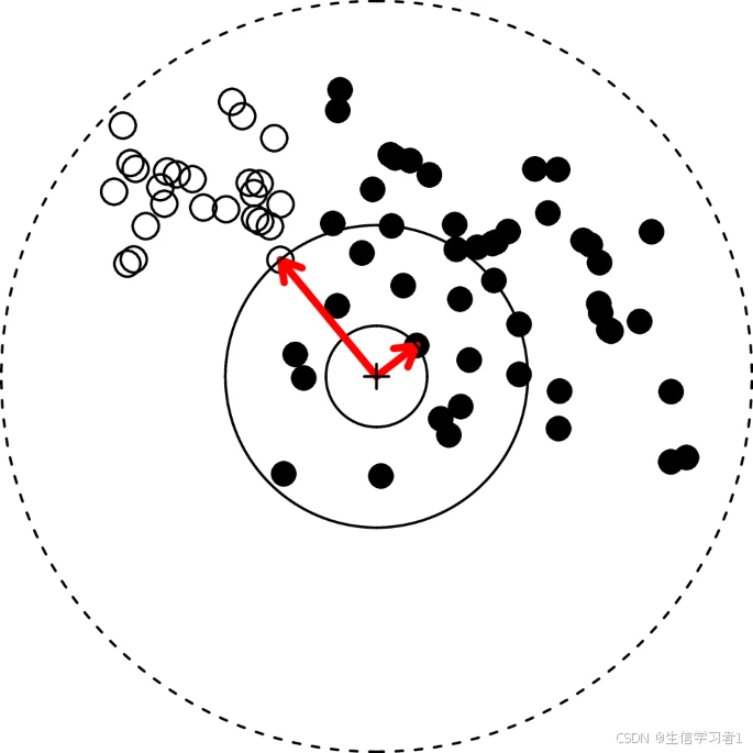
通过以递增规模的嵌套方式对不同区域内的物种数量进行计数而得出的嵌套物种 - 面积关系呈现出稳健且反复出现的定性和定量模式。当以双对数坐标系绘制时，它呈现出三个阶段：在小区域内的物种数量快速增长，在中间规模时增长速度较慢，在大区域时增长速度加快。尽管这一模式意义重大，但其理论基础仍不完全清楚。在此，我们利用极值理论为物种 - 面积关系构建了一个理论模型，并表明物种 - 面积关系是每个个体物种到起始采样焦点的最小距离分布的混合体。我们研究的一个关键见解是，每个阶段是由物种的地理分布（即它们的分布范围）相对于焦点点所决定的，这使我们能够开发出一个用于估算相变时物种数量的公式。我们通过将不同大陆和类群的实证物种 - 面积关系与使用全球生物多样性信息设施数据的预测进行比较来测试我们的方法。尽管 SAR 反映了组成物种的潜在生物学属性，但我们的解读和对极值理论的应用是具有普遍性的，并且能够广泛适用于具有类似空间特征的系统。

The nested species-area relationship, obtained by counting species in increasingly larger areas in a nested fashion, exhibits robust and recurring qualitative and quantitative patterns. When plotted in double logarithmic scales it shows three phases: rapid species increase at small areas, slower growth at intermediate scales, and faster rise at large scales. Despite its significance, the theoretical foundations of this pattern remain incompletely understood. Here, we develop a theory for the species-area relationship using extreme value theory, and show that the species-area relationship is a mixture of the distributions of minimum distances to a starting sampling focal point for each individual species. A key insight of our study is that each phase is determined by the geographical distributions of the species, i.e., their ranges, relative to the focal point, enabling us to develop a formula for estimating the number of species at phase transitions. We test our approach by comparing empirical species-area relationships for different continents and taxa with our predictions using Global Biodiversity Information Facility data. Although a SAR reflects the underlying biological attributes of the constituent species, our interpretations and use of the extreme value theory are general and can be widely applicable to systems with similar spatial features.

代码

https://zenodo.org/records/15269150

### Borda-de-Água et al. Extreme value theory explains the species-area relationship

### Created 17 May 2024, Luís Borda-de-Água

# Figure 1

# functions:

draw.circle <- function(R, lty, col = "black") {
  x <- seq(0.0, R, R / 1000)
  y <- sqrt(R^2 - x^2)

  lines(x, y, lty = lty, col = col)
  lines(x, -y, lty = lty, col = col)
  lines(-x, y, lty = lty, col = col)
  lines(-x, -y, lty = lty, col = col)
}

###

open_graphics_window <- function(width = 9, height = 5) {
  if (.Platform$OS.type == "windows") { # Windows
    windows(width = width, height = height)
  } else if (Sys.info()["sysname"] == "Darwin") { # Mac OS
    quartz(width = width, height = height)
  } else { # Assume Linux or Unix-like
    x11(width = width, height = height)
  }
}

###

plot.spp <- function(n, xmin, xmax, ymin, ymax, pch = 1, lty = 1) {
  x <- c(
    0.171891397, 0.111932677, 0.726411596, 0.8415692, 0.699219711, 0.454846982, 0.701518082, 0.562159697, 0.140375352,
    -0.004526590, -0.096394596, 0.169455724, 0.190195198, 0.704353367, 0.656949430, 0.089487327, 0.422342301, 0.060577829, 0.001633336, 0.588484763, 0.894380263, -0.119370967, 0.242476232, -0.006035809, 0.371303542, 0.272964170, 0.676368215, 0.732307641, 0.412740933, 0.593696158, 0.809483482, 0.150050425, 0.590720689, 0.324918679, 0.484301032, 0.416492280, 0.349924469, 0.527049762, -0.018190031, 0.295000653, 0.137009672, 0.893465236, 0.310720760, 0.208095286, 0.935758810, 0.326973883, 0.484379979, 0.314959719, -0.150431576, 0.152422304
  )

  y <- c(
    0.34482773, -0.16853769, 0.22593770, 0.4901067, 0.29633381, 0.49101054, 0.40671198, 0.54064082, 0.50588536, 0.81729414,
    0.09584226, 0.06461097, 0.68209353, 0.27152434, 0.46673673, 0.60441876, 0.46256030, 0.43296469, 0.87285586, 0.65784141, 0.05888994, 0.15938462, 0.64358169, 0.29009324, 0.44836678, -0.01434021, 0.45488172, 0.22203386, 0.45848244, 0.06036704, 0.24828992, 0.68929501, -0.04065262, 0.30841310, 0.24062768, 0.35878524, 0.14420193, 0.65942293, 0.51264159, -0.05801282, 0.69791648, -0.13046757, 0.50938987, 0.18340530, -0.11876154, 0.01870023, 0.10531118, 0.44275108, -0.16275379, 0.07577006
  )

  x <- x - 0.1
  y <- y - 0.1

  r <- sqrt(x^2 + y^2)
  x <- x[r < .975]
  y <- y[r < .975]
  r <- r[r < .975]

  x <- x[r > 0.1]
  y <- y[r > 0.1]
  r <- r[r > 0.1]

  pos.min <- which(r == min(r))
  pos.max <- which(r == max(r))

  par(mar = c(0, 0, 0, 0)) # changes the margins' size

  plot(x, y, xlim = c(-1, 1), ylim = c(-1, 1), xlab = "", ylab = "", xaxt = "n", yaxt = "n", pch = 20, cex = 3, axes = F)
  points(0, 0, pch = 3)

  arrows(0, 0, x[pos.min], y[pos.min], length = 0.1, col = "red")

  rmin <- min(r)
  draw.circle(rmin, 1)

  # Now add the second species

  x <- c(
    -0.3275178, -0.3310398, -0.7078598, -0.3154288, -0.3139587, -0.6843294, -0.3420654, -0.5723965, -0.6549125, -0.5649686, -0.2759476, -0.6720087,
    -0.4671133, -0.2874343, -0.6500376, -0.2593391, -0.4963501, -0.6639542, -0.5829321, -0.2589675, -0.4058235, -0.5388422, -0.3621775, -0.3898895,
    -0.6224721
  )
  y <- c(
    0.4258752, 0.4943471, 0.4981802, 0.5200116, 0.4178217, 0.6766097, 0.5221701, 0.4656546, 0.3155398, 0.5527994, 0.6427094, 0.3040067, 0.4554200,
    0.4050244, 0.5598147, 0.3144913, 0.5320593, 0.5753792, 0.5099927, 0.4643576, 0.4508025, 0.5445848, 0.7018757, 0.7405155, 0.4053569
  )

  points(x, y, cex = 2.5) # , pch=5)
  r <- sqrt(x^2 + y^2)

  pos.min <- which(r == min(r))
  pos.max <- which(r == max(r))

  arrows(0, 0, x[pos.min], y[pos.min], length = 0.1, col = "red")

  rmin <- min(r)
  draw.circle(rmin, 1)
  rmax <- max(r)
  draw.circle(rmax + 0.05, 2)
}

###

figure.1 <- function() {
  open_graphics_window(height = 6, width = 6)
  par(pty = "s")

  plot.spp(70, -.2, 1, -.2, 1, pch = 20, lty = 1)
}

figure.1()

参考

• Modelling the species-area relationship using extreme value theory