caffe学习:caffemodel可视化

网络架构的形象展示

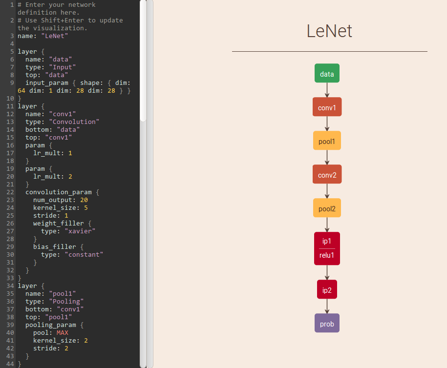
在构建完网络后, 我们得到一个xx_train.prototxt文件, 该文件中记录着每层网络的输入输出及规格等参数, 在地址http://ethereon.github.io/netscope/#/editor 左侧拖入xx_train.ptototxt文件, 按enter+shift组合键即可查看网络模型图, 非常具体形象.

以LeNet为例

# lenet.prototxt

name: "LeNet"

layer {
  name: "data"
  type: "Input"
  top: "data"
  input_param { shape: { dim: 64 dim: 1 dim: 28 dim: 28 } }
}
layer {
  name: "conv1"
  type: "Convolution"
  bottom: "data"
  top: "conv1"
  param {
    lr_mult: 1
  }
  param {
    lr_mult: 2
  }
  convolution_param {
    num_output: 20
    kernel_size: 5
    stride: 1
    weight_filler {
      type: "xavier"
    }
    bias_filler {
      type: "constant"
    }
  }
}
layer {
  name: "pool1"
  type: "Pooling"
  bottom: "conv1"
  top: "pool1"
  pooling_param {
    pool: MAX
    kernel_size: 2
    stride: 2
  }
}
layer {
  name: "conv2"
  type: "Convolution"
  bottom: "pool1"
  top: "conv2"
  param {
    lr_mult: 1
  }
  param {
    lr_mult: 2
  }
  convolution_param {
    num_output: 50
    kernel_size: 5
    stride: 1
    weight_filler {
      type: "xavier"
    }
    bias_filler {
      type: "constant"
    }
  }
}
layer {
  name: "pool2"
  type: "Pooling"
  bottom: "conv2"
  top: "pool2"
  pooling_param {
    pool: MAX
    kernel_size: 2
    stride: 2
  }
}
layer {
  name: "ip1"
  type: "InnerProduct"
  bottom: "pool2"
  top: "ip1"
  param {
    lr_mult: 1
  }
  param {
    lr_mult: 2
  }
  inner_product_param {
    num_output: 500
    weight_filler {
      type: "xavier"
    }
    bias_filler {
      type: "constant"
    }
  }
}
layer {
  name: "relu1"
  type: "ReLU"
  bottom: "ip1"
  top: "ip1"
}
layer {
  name: "ip2"
  type: "InnerProduct"
  bottom: "ip1"
  top: "ip2"
  param {
    lr_mult: 1
  }
  param {
    lr_mult: 2
  }
  inner_product_param {
    num_output: 10
    weight_filler {
      type: "xavier"
    }
    bias_filler {
      type: "constant"
    }
  }
}
layer {
  name: "prob"
  type: "Softmax"
  bottom: "ip2"
  top: "prob"
}

LeNet的网络架构:

网络模型参数的可视化

在**_solver.prototxt文件中, 通过设置snapshot参数来指定训练多少次后就保存一下当前训练的模型, 设置snapshot_prefix参数来指定模型保存的路径及文件名, 如xx_iter_5000.caffemodel.

在xx.caffemodel文件中存有各层的参数, 即net.params, 但是没有数据(net.blobs). 生成caffemodel文件的过程还会生成一个相应的solverstate文件, 这个solverstate文件与caffemodel相似, 但包含一些数据, 比如模型名称\当前迭代次数等.

两者的功能区别:
caffemodel是在测试阶段用于分类的
solverstate是用来恢复训练的, 为防止意外终止而保存的快照.

以LeNet为例

import numpy as np
import matplotlib.pyplot as plt
import os, sys
import caffe

caffe_root='/home/keysen/caffe/'
os.chdir(caffe_root)
sys.path.insert(0, caffe_root+'python')

#显示的图表大小为 8,图形的插值是以最近为原则,图像颜色是灰色
plt.rcParams['figure.figsize']=(8,8)
plt.rcParams['image.interpolation']='nearest'
plt.rcParams['image.cmap']='gray'

#设置网络为测试阶段，并加载网络模型prototxt和已训练网络caffemodel文件
net = caffe.Net(caffe_root + 'examples/mnist/lenet_train_test.prototxt',
                caffe_root + 'examples/mnist/lenet_iter_10000.caffemodel',
                caffe.TEST)
[(k, v[0].data.shape) for k, v in net.params.items()]

#可视化的辅助函数
#take an array of shape (n, height, width) or (n, height, width, channels)用一个格式是(数量,高,宽)或(数量,高,宽,频道)的阵列
#and visualize each (height, width) thing in a grid of size approx. sqrt(n) by sqrt(n)每个可视化的都是在一个由一个个网格组
#编写一个函数，用于显示各层的参数
def show_feature(data, padsize=1, padval=0):
    data -= data.min()
    data /= data.max()

    # force the number of filters to be square
    n = int(np.ceil(np.sqrt(data.shape[0])))
    padding = ((0, n ** 2 - data.shape[0]), (0, padsize), (0, padsize)) + ((0, 0),) * (data.ndim - 3)
    data = np.pad(data, padding, mode='constant', constant_values=(padval, padval))
    print data.shape

    # tile the filters into an image
    data = data.reshape((n, n) + data.shape[1:]).transpose((0, 2, 1, 3) + tuple(range(4, data.ndim + 1)))
    print data.shape
    data = data.reshape((n * data.shape[1], n * data.shape[3]) + data.shape[4:])
    print data.shape
    plt.imshow(data)
    plt.axis('off')
    plt.show()

output:

[(‘conv1’, (50, 1, 5, 5)),
(‘conv2’, (20, 50, 5, 5)),
(‘ip1’, (512, 320)),
(‘ip2’, (10, 512))]

#根据每一层的名称，选择需要可视化的层，可以可视化filter（参数）
# the parameters are a list of [weights, biases],各层的特征
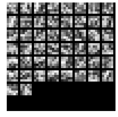
# 第一个卷积层，参数规模为(20,1,5,5)，即20个5*5的1通道filter
weight = net.params["conv1"][0].data
print weight.shape
show_feature(weight.reshape(weight.shape[0]*weight.shape[1], 5, 5))
#show_feature(weight.transpose(0, 2, 3, 1))

output

(50, 1, 5, 5)
(64, 6, 6)
(8, 6, 8, 6)
(48, 48)

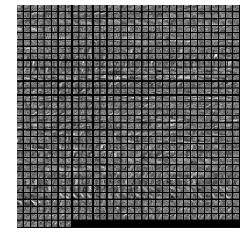
# 第二个卷积层的权值参数，共有50*20个filter,每个filter大小为5*5
weight = net.params["conv2"][0].data
print weight.shape
show_feature(weight.reshape(weight.shape[0]*weight.shape[1], 5, 5))

output:

(20, 50, 5, 5)
(1024, 6, 6)
(32, 6, 32, 6)
(192, 192)

另附一篇详细的相关博客,可参考caffe 提取特征并可视化（已测试可执行）及在线可视化