


一、自编码器
任务描述
本关任务:搭建一个简单的自编码器模型。
相关知识
为了完成本关任务,你需要掌握:1.基本的自编码概念,2.搭建简单的自编码器模型。
自编码器
自编码器简介
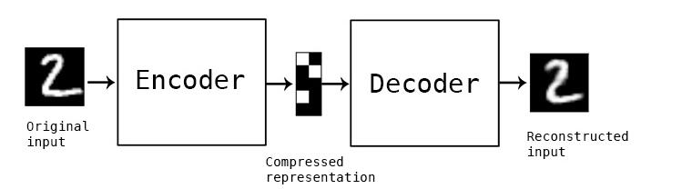
自编码器是一类尝试使用反向传播算法重新创建输入数据作为输出的神经网络。自编码器包含两部分:编码器和解码器。编码器读取输入并把它压缩成紧凑表示,解码器则读取紧凑表示并用其重建输入。如下图所示:
搭建简单的自编码器模型
可以通过keras很快的创建如下的编码器和解码器并编译,代码如下:
from keras.layers import Input, Densefrom keras.models import Model# 编码器维度encoding_dim = 32input_img = Input(shape=(784,))# "encoded" 是把输入编码表示encoded = Dense(encoding_dim, activation='relu')(input_img)# "decoded" 是输入的有损重构decoded = Dense(784, activation='sigmoid')(encoded)# 搭建自编码模型autoencoder = Model(input_img, decoded)autoencoder.compile(optimizer='adadelta', loss='binary_crossentropy')# 打印模型结构autoencoder.summary()
运行结果:
_________________________________________________________________Layer (type) Output Shape Param #=================================================================input_1 (InputLayer) (None, 784) 0_________________________________________________________________dense_1 (Dense) (None, 32) 25120_________________________________________________________________dense_2 (Dense) (None, 784) 25872=================================================================Total params: 50,992Trainable params: 50,992Non-trainable params: 0_________________________________________________________________
导入数据集
可通过以下代码导入mnist数据集,代码如下:
from keras.datasets import mnistimport numpy as np# 加载数据集(x_train, _), (x_test, _) = mnist.load_data()# 对图片数据进行归一化x_train = x_train.astype('float32') / 255.x_test = x_test.astype('float32') / 255.# 转换数据形状x_train=x_train.reshape((len(x_train),np.prod(x_train.shape[1:]))x_test =x_test.reshape((len(x_test), np.prod(x_test.shape[1:])))print(x_train.shape)print(x_test.shape)
运行结果:
(60000,784)(10000,784)
拟合模型
通过以上数据拟合模型autoencoder,提示:epochs =50,batch_size=256,shuffle=True 。 代码如下:
autoencoder.fit(x_train, x_train,epochs=50,batch_size=256,shuffle=True,validation_data=(x_test, x_test))
代码执行结果:
Train on 60000 samples, validate on 10000 samplesEpoch 1/5060000/60000 [==============================] - 5s 83us/step - loss: 0.3567 - val_loss: 0.2714Epoch 2/5060000/60000 [==============================] - 4s 61us/step - loss: 0.2645 - val_loss: 0.2545Epoch 3/5060000/60000 [==============================] - 4s 61us/step - loss: 0.2450 - val_loss: 0.2333Epoch 4/5060000/60000 [==============================] - 4s 62us/step - loss: 0.2248 - val_loss: 0.2139Epoch 5/5060000/60000 [==============================] - 4s 61us/step - loss: 0.2078 - val_loss: 0.1997…60000/60000 [==============================] - 4s 73us/step - loss: 0.1055 - val_loss: 0.1037Epoch 50/5060000/60000 [==============================] - 4s 75us/step - loss: 0.1052 - val_loss: 0.1033
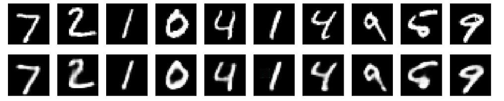
查看重构的输出与原来的输出对比
我们可以通过以下方式来查看,代码如下:
# 从测试集选取一些数据来编码和解码encoded_imgs = encoder.predict(x_test)decoded_imgs = decoder.predict(encoded_imgs)import matplotlib.pyplot as pltn = 10 # 打印的图片数量plt.figure(figsize=(20, 4))for i in range(n):# 显示原来图像ax = plt.subplot(2, n, i + 1)plt.imshow(x_test[i].reshape(28, 28))plt.gray()ax.get_xaxis().set_visible(False)ax.get_yaxis().set_visible(False)# 显示重构后的图像ax = plt.subplot(2, n, i + 1 + n)plt.imshow(decoded_imgs[i].reshape(28, 28))plt.gray()ax.get_xaxis().set_visible(False)ax.get_yaxis().set_visible(False)plt.show()
代码执行结果:

编程要求
根据左侧内容提示,补充右侧代码部分内容。
- 补充训练自编码器模型代码。
- 补充编码器模型参数。
因评测时间限时,实战代码只训练五轮的结果进行评测对比。
测试说明
平台会对你编写的代码进行测试:
测试输入:略; 预期输出: 通关成功!
开始你的任务吧,祝你成功!
代码部分
from keras.layers import Input, Dense, Conv2D, MaxPooling2D, UpSampling2D
from keras.models import Model
from Keras.datasets import mnist
import numpy as np
import matplotlib.pyplot as plt

# 设置随机种子
np.random.seed(1447)


def draw(X_test, decoded_imgs):
    # 打印图片的数量
    n = 10
    # 画布大小
    plt.figure(figsize=(20, 4))
    for i in range(n):
        ax = plt.subplot(2, n, i+1)
        plt.imshow(X_test[i].reshape(28, 28))
        plt.gray()
        ax.get_xaxis().set_visible(False)
        ax.get_yaxis().set_visible(False)
        # 显示重构之后的图像
        ax = plt.subplot(2, n, i+1+n)
        plt.imshow(decoded_imgs[i].reshape(28, 28))
        plt.gray()
        ax.get_xaxis().set_visible(False)
        ax.get_yaxis().set_visible(False)

    # 保存图片文件
    plt.savefig("src/step1/stu_img/result.png")
    plt.show()


def autoencoder1():
    # 编码器维度
    encoding_dim = 32
    input_img = Input(shape=(784,))
    # "encoded" 是把输入编码表示
    encoded = Dense(encoding_dim, activation='relu')(input_img)
    # "decoded" 是输入的有损重构
    decoded = Dense(784, activation='sigmoid')(encoded)

    # 自编码模型
    autoencoder = Model(input_img, decoded)
    autoencoder.compile(optimizer='adadelta', loss='binary_crossentropy')

    # 加载数据
    (X_train, _), (X_test, _) = mnist.load_data()
    # 数据归一化
    X_train = X_train.astype('float32') / 255
    X_test = X_test.astype('float32') / 255
    # 形状转换
    X_train = X_train.reshape((len(X_train), np.prod(X_train.shape[1:])))
    X_test = X_test.reshape((len(X_test), np.prod(X_test.shape[1:])))
    print(X_train.shape)
    print(X_test.shape)

    # 训练模型参数,补充下面代码
    # 训练5轮,batch_size设置为5,shuffle为True。
    # validation_data放入测试集数据,verbose设置为2则不输出进度条。
    # ********** Begin *********#


    # autoencoder.fit( )

    autoencoder.fit(X_train, X_train,
                epochs=5,
                batch_size=256,
                shuffle=True,
                validation_data=(X_test, X_test),
                verbose=2
                )
    # ********** End **********#

    # 获取编码器和解码器

    # ********** Begin *********#
    # "encoded" 是把输入编码表示,补充下面代码
    # encoder = Model(inputs=, outputs=)
    # encoded_input = Input(shape=(encoding_dim,))
    encoder = Model(inputs=input_img, outputs=encoded)
    encoded_input = Input(shape=(encoding_dim,))
    # ********** End **********#
    # "decoded" 是输入的有损重构
    decoder_layer = autoencoder.layers[-1]
    decoder = Model(inputs=encoded_input, outputs=decoder_layer(encoded_input))

    # 预测
    encoded_imgs = encoder.predict(X_test)
    decoded_imgs = decoder.predict(encoded_imgs)
    # 显示
    draw(X_test, decoded_imgs)
二、卷积自编码器
任务描述
本关任务:编写一个卷积自编码器。
相关知识
为了完成本关任务,你需要掌握:1.卷积自编码器的基础知识,2.使用keras实现卷积自编码器。
卷积自编码器
搭建卷积自编码器
当输入是图像时,使用卷积神经网络基本上总是有意义的。在现实中,用于处理图像的自动编码器几乎都是卷积自动编码器——又简单又快。 卷积自编码器的编码器部分由卷积层和MaxPooling层构成,MaxPooling负责空域下采样。而解码器由卷积层和上采样层构成。
我们可以通过以下方式来创建如下的卷积编码器和解码器并编译,代码如下:
from keras.layers import Input, Dense, Conv2D, MaxPooling2D, UpSampling2Dfrom keras.models import Modelfrom keras import backend as Kinput_img = Input(shape=(28, 28, 1)) #输入图像形状#编码器x=Conv2D(16, (3, 3), activation='relu', padding='same')(input_img)#卷积层x = MaxPooling2D((2, 2), padding='same')(x)#空域下采样x = Conv2D(8, (3, 3), activation='relu', padding='same')(x)x = MaxPooling2D((2, 2), padding='same')(x)x = Conv2D(8, (3, 3), activation='relu', padding='same')(x)encoded = MaxPooling2D((2, 2), padding='same')(x)#解码x = Conv2D(8, (3, 3), activation='relu', padding='same')(encoded)x = UpSampling2D((2, 2))(x)#上采样层x = Conv2D(8, (3, 3), activation='relu', padding='same')(x)x = UpSampling2D((2, 2))(x)x = Conv2D(16, (3, 3), activation='relu')(x)x = UpSampling2D((2, 2))(x)decoded = Conv2D(1, (3, 3), activation='sigmoid', padding='same')(x)# 定义模型autoencoder = Model(input_img, decoded)# 编译模型autoencoder.compile(optimizer='adadelta', loss='binary_crossentropy')#编译# 打印模型结构autoencoder.summary()
运行结果:
_________________________________________________________________Layer (type) Output Shape Param #=================================================================input_1 (InputLayer) (None, 28, 28, 1) 0_________________________________________________________________conv2d_1 (Conv2D) (None, 28, 28, 16) 160_________________________________________________________________max_pooling2d_1 (MaxPooling2 (None, 14, 14, 16) 0_________________________________________________________________conv2d_2 (Conv2D) (None, 14, 14, 8) 1160_________________________________________________________________max_pooling2d_2 (MaxPooling2 (None, 7, 7, 8) 0_________________________________________________________________conv2d_3 (Conv2D) (None, 7, 7, 8) 584_________________________________________________________________max_pooling2d_3 (MaxPooling2 (None, 4, 4, 8) 0_________________________________________________________________conv2d_4 (Conv2D) (None, 4, 4, 8) 584_________________________________________________________________up_sampling2d_1 (UpSampling2 (None, 8, 8, 8) 0_________________________________________________________________conv2d_5 (Conv2D) (None, 8, 8, 8) 584_________________________________________________________________up_sampling2d_2 (UpSampling2 (None, 16, 16, 8) 0_________________________________________________________________conv2d_6 (Conv2D) (None, 14, 14, 16) 1168_________________________________________________________________up_sampling2d_3 (UpSampling2 (None, 28, 28, 16) 0_________________________________________________________________conv2d_7 (Conv2D) (None, 28, 28, 1) 145=================================================================Total params: 4,385Trainable params: 4,385Non-trainable params: 0_________________________________________________________________Process finished with exit code 0
加载数据并拟合模型
请参考上个关卡加载数据并完成模型拟合。 提示1:
x_train 用 reshape重构时参数设置为 x_train = np.reshape(x_train, (len(x_train), 28, 28, 1)) ,x_test 同上类似。
提示2:
autoencoder 中的 batch_size 设置为 128,其他不变。
代码如下:
from keras.datasets import mnistimport numpy as np# 加载数据(x_train, _), (x_test, _) = mnist.load_data()# 归一化x_train = x_train.astype('float32') / 255.x_test = x_test.astype('float32') / 255.# 转换形状x_train = np.reshape(x_train, (len(x_train), 28, 28, 1))x_test = np.reshape(x_test, (len(x_test), 28, 28, 1))# 训练模型autoencoder.fit(x_train, x_train,epochs=50,batch_size=128,shuffle=True,validation_data=(x_test, x_test),)
运行结果:
Train on 60000 samples, validate on 10000 samplesEpoch 1/5060000/60000 [==============================] - 42s 699us/step - loss: 0.2094 - val_loss: 0.1738Epoch 2/5060000/60000 [==============================] - 35s 586us/step - loss: 0.1511 - val_loss: 0.1389Epoch 3/5060000/60000 [==============================] - 36s 603us/step - loss: 0.1371 - val_loss: 0.1302Epoch 4/5060000/60000 [==============================] - 36s 604us/step - loss: 0.1301 - val_loss: 0.1256Epoch 5/5060000/60000 [==============================] - 37s 609us/step - loss: 0.1256 - val_loss: 0.1236…Epoch 49/5060000/60000 [==============================] - 38s 633us/step - loss: 0.0981 - val_loss: 0.0951Epoch 50/5060000/60000 [==============================] - 39s 644us/step - loss: 0.0979 - val_loss: 0.0953<keras.callbacks.History at 0x7fbec2d90128>
查看重构的输出与原来的输出对比
查看 10 张重构后的图像与原图像的对比。 代码如下:
# 预测decoded_imgs = autoencoder.predict(x_test)n = 10plt.figure(figsize=(20, 4))for i in range(n):# 显示原图像ax = plt.subplot(2, n, i+1)plt.imshow(x_test[i].reshape(28, 28))plt.gray()ax.get_xaxis().set_visible(False)ax.get_yaxis().set_visible(False)# 显示重构后的图像ax = plt.subplot(2, n, i + n+1)plt.imshow(decoded_imgs[i].reshape(28, 28))plt.gray()ax.get_xaxis().set_visible(False)ax.get_yaxis().set_visible(False)plt.show()
运行结果:
编程要求
根据左侧内容提示,补充右侧代码部分内容。
- 补充编码器模型的卷积层和最大池化层参数。
- 补充解码器模型的上采样层和卷积层参数。
因评测时间限时,实战代码只训练五轮的结果进行评测对比。
测试说明
平台会对你编写的代码进行测试:
测试输入:略; 预期输出: 通关成功!
开始你的任务吧,祝你成功!
代码部分
from keras.layers import Input, Dense, Conv2D, MaxPooling2D, UpSampling2D
from keras.models import Model
from Keras.datasets import mnist
import numpy as np
import matplotlib.pyplot as plt

# 设置随机种子
np.random.seed(1447)


def draw(X_test, decoded_imgs):

    n = 10
    plt.figure(figsize=(20, 4))
    for i in range(n):
        ax = plt.subplot(2, n, i+1)
        plt.imshow(X_test[i].reshape(28, 28))
        plt.gray()
        ax.get_xaxis().set_visible(False)
        ax.get_yaxis().set_visible(False)
        # 显示重构之后的图像
        ax = plt.subplot(2, n, i+1+n)
        plt.imshow(decoded_imgs[i].reshape(28, 28))
        plt.gray()
        ax.get_xaxis().set_visible(False)
        ax.get_yaxis().set_visible(False)
    plt.savefig("src/step2/stu_img/result.png")
    plt.show()


def autoencoder2():
    # 卷积编码器
    input_img = Input(shape=(28, 28, 1))  # 输入图像形状
    ###编码器
    # 卷积层
    x = Conv2D(16, (3, 3), activation='relu', padding='same')(input_img)
    # 最大池化
    x = MaxPooling2D((2, 2), padding='same')(x)

    x = Conv2D(8, (3, 3), activation='relu', padding='same')(x)
    x = MaxPooling2D((2, 2), padding='same')(x)

    # 定义一个卷积,卷积核大小为8,形状为(3,3),激活函数为relu,padding为same
    # encoded是最大池化,池化形状为(2,2),padding为same
    # ********** Begin *********#
    # x =
    # encoded =
    x = Conv2D(8, (3, 3), activation='relu', padding='same')(x)
    encoded = MaxPooling2D((2, 2), padding='same')(x)
    # ********** End *********#

    ###解码器
    x = Conv2D(8, (3, 3), activation='relu', padding='same')(encoded)
    # 上采样层
    x = UpSampling2D((2, 2))(x)
    x = Conv2D(8, (3, 3), activation='relu', padding='same')(x)
    x = UpSampling2D((2, 2))(x)
    x = Conv2D(16, (3, 3), activation='relu')(x)

    # 定义一个上采样层,形状为(2,2)
    # decoded是卷积层,卷积核大小为1,形状为(3,3),激活函数为sigmoid,padding为same
    # ********** Begin *********#
    # x =
    # decoded =
    x = UpSampling2D((2, 2))(x)
    decoded = Conv2D(1, (3, 3), activation='sigmoid', padding='same')(x)

    # ********** Begin *********#


    autoencoder = Model(input_img, decoded)
    autoencoder.compile(optimizer='adadelta', loss='binary_crossentropy')

    # 数据处理
    (X_train, _), (X_test, _) = mnist.load_data()
    # 数据归一化
    X_train = X_train.astype('float32') / 255
    X_test = X_test.astype('float32') / 255
    # 数据形状转换
    X_train = np.reshape(X_train, (len(X_train), 28, 28, 1))
    X_test = np.reshape(X_test, (len(X_test), 28, 28, 1))
    print(X_train.shape)
    print(X_test.shape)

    # 训练模型
    autoencoder.fit(X_train, X_train, epochs=5, batch_size=128,
                    shuffle=True, validation_data=(X_test, X_test))
    # 预测
    decoded_imgs = autoencoder.predict(X_test)
    # 显示
    draw(X_test, decoded_imgs)
三、自编码器的应用
任务描述
本关任务:对数据集加入噪点,构建自编码器。
相关知识
为了完成本关任务,你需要掌握:1.自编码器在数据加入噪点后进行还原,2.编写代码进行实现。
自编码器的应用
介绍
我们把训练样本用噪声污染,然后使用解码器解码出干净的照片,以获得去噪自动编码器。
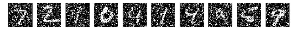
把原图片加入高斯噪声
我们可以通过以下方式来加入噪声并查看加噪后的图片,代码如下:
from keras.datasets import mnistimport numpy as np# 加载数据(x_train, _), (x_test, _) = mnist.load_data()# 归一化x_train = x_train.astype('float32') / 255.x_test = x_test.astype('float32') / 255.# 形状转换x_train = np.reshape(x_train, (len(x_train), 28, 28, 1))x_test = np.reshape(x_test, (len(x_test), 28, 28, 1))noise_factor = 0.5# 噪点x_train_noisy = x_train + noise_factor * np.random.normal(loc=0.0, scale=1.0, size=x_train.shape)x_test_noisy = x_test + noise_factor * np.random.normal(loc=0.0, scale=1.0, size=x_test.shape)x_train_noisy = np.clip(x_train_noisy, 0., 1.)x_test_noisy = np.clip(x_test_noisy, 0., 1.)n = 10plt.figure(figsize=(20, 2))# 显示for i in range(n):ax = plt.subplot(1, n, i+1)plt.imshow(x_test_noisy[i].reshape(28, 28))plt.gray()ax.get_xaxis().set_visible(False)ax.get_yaxis().set_visible(False)plt.show()
代码执行结果:
构建自编码器
参考上一关卡按如下步骤使用Keras函数模型搭建自编码器并拟合。
1)设置input_img参数。 2)搭建编码器,添加Conv2D层,输入是input_img,输出维度 32,卷积核大小3×3,激活函数’‘relu’,padding设置为‘same’,返回给x。 3)添加Maxpooling2D层,大小是(2,2),padding设置为‘same’。 4)添加Conv2D层,输出维度 32,卷积核大小3×3,激活函数’‘relu’,padding设置为‘same’。 5)添加Maxpooling2D层,大小是(2,2),padding设置为‘same’,返回给encoded。 6)设置解码器,添加Conv2D层,输入是encoded,输出维度 32,卷积核大小3×3,激活函数’‘relu’,padding设置为‘same’,返回给x。 7)添加上采样层,大小是(2,2)。 8)添加Conv2D层,输出维度 32,卷积核大小3×3,激活函数’‘relu’,padding设置为‘same’。 9)添加上采样层,大小是(2,2)。 10)添加Conv2D层,输入是encoded,输出维度 1,卷积核大小3×3,激活函数’‘sigmoid’,padding设置为‘same’,返回给decoded。 11)设置自编码器,输入是input_img,decoded。 12)编译自编码器,参数不变。 13)拟合数据,参数与上个关卡一样。
# 输入尺寸input_img = Input(shape=(28, 28, 1))# 卷积层x = Conv2D(32, (3, 3), activation='relu', padding='same')(input_img)# 池化层x = MaxPooling2D((2, 2), padding='same')(x)x = Conv2D(32, (3, 3), activation='relu', padding='same')(x)encoded = MaxPooling2D((2, 2), padding='same')(x)# 卷积层x = Conv2D(32, (3, 3), activation='relu', padding='same')(encoded)# 上采样层x = UpSampling2D((2, 2))(x)x = Conv2D(32, (3, 3), activation='relu', padding='same')(x)x = UpSampling2D((2, 2))(x)decoded = Conv2D(1, (3, 3), activation='sigmoid', padding='same')(x)# 定义模型autoencoder = Model(input_img, decoded)# 模型编译autoencoder.compile(optimizer='adadelta', loss='binary_crossentropy')# 训练模型autoencoder.fit(x_train_noisy, x_train,epochs=100,batch_size=128,shuffle=True,validation_data=(x_test_noisy, x_test),)
代码执行结果:
Train on 60000 samples, validate on 10000 samplesEpoch 1/5060000/60000 [==============================] - 66s 1ms/step - loss: 0.1182 - val_loss: 0.1111Epoch 2/5060000/60000 [==============================] - 63s 1ms/step - loss: 0.1114 - val_loss: 0.1081Epoch 3/5060000/60000 [==============================] - 71s 1ms/step - loss: 0.1077 - val_loss: 0.1035Epoch 4/5060000/60000 [==============================] - 71s 1ms/step - loss: 0.1055 - val_loss: 0.1034Epoch 5/5060000/60000 [==============================] - 60s 1ms/step - loss: 0.1040 - val_loss: 0.1036…Epoch 49/5060000/60000 [==============================] - 68s 1ms/step - loss: 0.0954 - val_loss: 0.0950Epoch 50/5060000/60000 [==============================] - 67s 1ms/step - loss: 0.0953 - val_loss: 0.0946<keras.callbacks.History at 0x7f685ce82390>
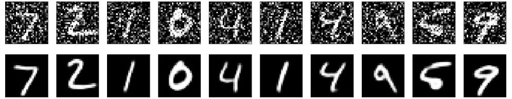
查看重构的输出与原来的输出对比
查看10张重构后的图像与原图像的对比。
代码如下:
# 预测decoded_imgs = autoencoder.predict(x_test)n = 10plt.figure(figsize=(20, 4))# 显示10张重构后的图像与原图像的对比for i in range(n):ax = plt.subplot(2, n, i + 1)plt.imshow(x_test_noisy[i].reshape(28, 28))plt.gray()ax.get_xaxis().set_visible(False)ax.get_yaxis().set_visible(False)ax = plt.subplot(2, n, i + n + 1)plt.imshow(decoded_imgs[i].reshape(28, 28))plt.gray()ax.get_xaxis().set_visible(False)ax.get_yaxis().set_visible(False)plt.show()
执行代码结果:
编程要求
根据左侧内容提示,补充右侧代码部分内容。
- 补充对测试集数据的噪点和截取操作。
- 补充自编码器模型的编译参数。
因评测时间限时,实战代码只训练十轮的结果进行评测对比。
测试说明
平台会对你编写的代码进行测试:
测试输入:略; 预期输出: 通关成功!
开始你的任务吧,祝你成功!
代码部分
from keras.layers import Input, Dense, Conv2D, MaxPooling2D, UpSampling2D
from keras.models import Model
from Keras.datasets import mnist
import numpy as np
import matplotlib.pyplot as plt

# 设置随机种子
np.random.seed(1447)


def draw(X_test, decoded_imgs):
    n = 10
    plt.figure(figsize=(20, 4))
    for i in range(n):
        ax = plt.subplot(2, n, i+1)
        plt.imshow(X_test[i].reshape(28, 28))
        plt.gray()
        ax.get_xaxis().set_visible(False)
        ax.get_yaxis().set_visible(False)
        # 显示重构之后的图像
        ax = plt.subplot(2, n, i+1+n)
        plt.imshow(decoded_imgs[i].reshape(28, 28))
        plt.gray()
        ax.get_xaxis().set_visible(False)
        ax.get_yaxis().set_visible(False)

    # 保存图片文件
    plt.savefig("src/step3/stu_img/result.png")
    plt.show()


def autoencoder3():
    # 数据处理
    (X_train, _), (X_test, _) = mnist.load_data()
    # 数据归一化
    X_train = X_train.astype('float32') / 255
    X_test = X_test.astype('float32') / 255
    # 数据形状转换
    X_train = np.reshape(X_train, (len(X_train), 28, 28, 1))
    X_test = np.reshape(X_test, (len(X_test), 28, 28, 1))

    # 加入数据噪点
    # ********** Begin *********#

    noise_factor = 0.5  # 噪点因子
    X_train_noisy = X_train + noise_factor * np.random.normal(loc=0.0, scale=1.0, size=X_train.shape)

    # 给测试集加入噪点
    #X_test_noisy =
    X_test_noisy = X_test + noise_factor * np.random.normal(loc=0.0, scale=1.0, size=X_test.shape)
    X_train_noisy = np.clip(X_train_noisy, 0., 1.)

    # 对测试集进行截取
    # X_test_noisy =
    X_test_noisy = np.clip(X_test_noisy, 0., 1.)
    # ********** End *********#


    # 输入图片形状
    input_img = Input(shape=(28, 28, 1))
    ### 编码器
    x = Conv2D(32, (3, 3), activation='relu', padding='same')(input_img)
    x = MaxPooling2D((2, 2), padding='same')(x)
    x = Conv2D(32, (3, 3), activation='relu', padding='same')(x)
    encoded = MaxPooling2D((2, 2), padding='same')(x)

    ### 解码器
    x = Conv2D(32, (3, 3), activation='relu', padding='same')(encoded)
    x = UpSampling2D((2, 2))(x)
    x = Conv2D(32, (3, 3), activation='relu', padding='same')(x)
    x = UpSampling2D((2, 2))(x)
    decoded = Conv2D(1, (3, 3), activation='sigmoid', padding='same')(x)

    # 定义模型
    autoencoder = Model(input_img, decoded)

    # 编译模型,优化器为adadelta,损失函数为binary_crossentropy
    # ********** Begin *********#
    # autoencoder.compile()
    autoencoder.compile(optimizer='adadelta', loss='binary_crossentropy')

    # ********** End *********#

    # 训练模型
    autoencoder.fit(X_train_noisy, X_train, epochs=10, batch_size=128,
                    shuffle=True, validation_data=(X_test_noisy, X_test))

    # 预测
    decoded_imgs = autoencoder.predict(X_test)
    # 显示
    draw(X_test_noisy, decoded_imgs)


 被折叠的 条评论
为什么被折叠?
被折叠的 条评论
为什么被折叠?
 到【灌水乐园】发言


