利用pytorch实现Fooling Images(添加特定噪声到原始图像,使神经网络误识别)

It suggests that it is the space, rather than the individual units, that contains the semantic information in the high layers of neural networks.
在深层的神经网络中，真正影响特征信息的，不是个体单元，而是空间信息。
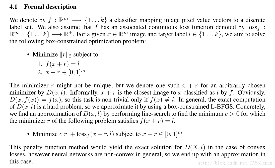
we find that deep neural networks learn input-output mappings that are fairly discontinuous to a significant extent.
神经网络对输入图像的分析是不连续的，所以通过这个特点可以在原始图像上加上一种特定噪声来实现误导
These results suggest that the deep neural networks that are learned by backpropagation have nonintuitive characteristics and intrinsic blind spots, whose structure is connected to the data distribution in a non-obvious way.
这些分析中可以得到深度学习网络通过反向传播学习到的数据拥有非直接的特性，还有一些固有的盲点，这些数据的结构与数据的分布有着隐秘的关系。

Fooling Images

fooling images，顾名思义，就是指一张图片，虽然上面通过肉眼看到的是松鼠（举个例子），但是因为这张图片加了一些特定的噪声，所以神经网络会将它误识别为其他物体。

理论基础

下面程序定义了一个生成fooling image 的函数。

def make_fooling_image(X, target_y, model):
    """
    生成一个与输入图像X类似的fooling image, 但是这个image会被分类成target_y.

    Inputs:
    - X: Input image; Tensor of shape (1, 3, 224, 224)
    - target_y: An integer in the range [0, 1000)
    - model: A pretrained CNN

    Returns:
    - X_fooling: An image that is close to X, but that is classifed as target_y
    by the model.
    """
    # Initialize our fooling image to the input image, and wrap it in a Variable.
    X_fooling = X.clone()
    X_fooling_var = Variable(X_fooling, requires_grad=True)

    learning_rate = 0.8
    ##############################################################################
    # TODO: Generate a fooling image X_fooling that the model will classify as   #
    # the class target_y. You should perform gradient ascent on the score of the #
    # target class, stopping when the model is fooled.  
    # 通过对目标分类的梯度更新直到该图像被模型误分为target_y
    # When computing an update step, first normalize the gradient:               #
    #   dX = learning_rate * g / ||g||_2                                         #
    #                                                                            #
    # You should write a training loop.                                          #
    #                                                                            #
    # HINT: For most examples, you should be able to generate a fooling image    #
    # in fewer than 100 iterations of gradient ascent.                           #
    # You can print your progress over iterations to check your algorithm.       #
    ##############################################################################
     for i in range(100):

            # 前向操作
            scores = model(X_fooling_var)
    #         print(scores)

            # Current max index.
            _, index = scores.data.max(dim=1)
            print(index)

            # 当成功fool的时候break.
            if index[0] == target_y:
                break

            # Score for the target class.
            target_score = scores[0,target_y]

            # Backward.
            target_score.backward()

            # Gradient for image.
            im_grad = X_fooling_var.grad.data

            # 通过正则化的梯度对所输入图像进行更新.
            X_fooling_var.data += learning_rate * (im_grad / im_grad.norm()) 

            # 梯度更新清零，否则梯度会进行累积.
            X_fooling_var.grad.data.zero_()

    return X_fooling

接下来运行函数来生成fooling image，具体信息通过上下文来观察。

idx = 0
target_y = 6

X_tensor = torch.cat([preprocess(Image.fromarray(x)) for x in X], dim=0)
X_fooling = make_fooling_image(X_tensor[idx:idx+1], target_y, model)

scores = model(Variable(X_fooling))
# print(target_y)
# print(scores.data.max(dim=1)[1])
assert target_y == scores.data.max(dim=1)[1][0], 'The model is not fooled!'

展示fooling image与识别结果

X_fooling_np = deprocess(X_fooling.clone())
X_fooling_np = np.asarray(X_fooling_np).astype(np.uint8)

plt.subplot(1, 4, 1)
plt.imshow(X[idx])
plt.title(class_names[y[idx]])
plt.axis('off')

plt.subplot(1, 4, 2)
plt.imshow(X_fooling_np)
plt.title(class_names[target_y])
plt.axis('off')

plt.subplot(1, 4, 3)
X_pre = preprocess(Image.fromarray(X[idx]))
diff = np.asarray(deprocess(X_fooling - X_pre, should_rescale=False))
plt.imshow(diff)
plt.title('Difference')
plt.axis('off')

plt.subplot(1, 4, 4)
diff = np.asarray(deprocess(10 * (X_fooling - X_pre), should_rescale=False))
plt.imshow(diff)
plt.title('Magnified difference (10x)')
plt.axis('off')

plt.gcf().set_size_inches(12, 5)
plt.show()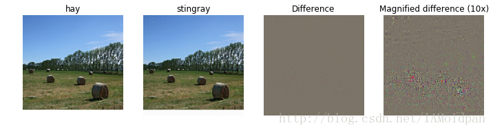

可以看出，hay图像被误识别为stinggray，而这两个图片的区别通过放大可以观察出random噪声。

参考资料：
Szegedy et al, “Intriguing properties of neural networks”, ICLR 2014
cs231n