【促销定价】背后的算法技术5-运筹决策模型

运筹匠心

于 2024-03-24 10:23:00 发布

阅读量1.1k

点赞数 18

分类专栏：促销定价文章标签：算法数学建模人工智能 python 数据挖掘

本文链接：https://blog.csdn.net/IndustryOR/article/details/136983206

版权

促销定价专栏收录该内容

6 篇文章 4 订阅

订阅专栏

导读：本篇是【促销定价】系列5篇文章的最后一篇。用5篇文章，我们系统介绍了如何将一个实际的促销定问题转化为一个数学问题，并利用数据预处理与挖掘、统计学与机器学习、运筹优化等技术从 0-1 的解决该问题。帮助大家对定价算法落地应用有了一个基本的认识，为后续的深入学习奠定基础。

作者 1：张哲铭，算法专家，某互联网大厂
作者 2：向杜兵，算法专家，某制造业龙头

明人不说暗话，【运筹匠心】想要大家的赞！赞！赞！。先赞后看，多多益善(*￣︶￣)~~~
本期推文代码获取方式，将推文转发朋友圈获20赞，截图发后台，管理员会定期回复数据代码连接哈~~~
各个系列的开源资料会定期整理发放，大家可以加粉丝群领取哦~~~

粉丝1群二维码：

加不了群，请加管理员微信：IndustryOR

大家好！我们是IndustryOR 团队，致力于分享业界落地的OR+AI技术。欢迎关注微信公众号/知乎【运筹匠心】 。本期我们来谈一谈《促销定价背后的算法技术》。促销活动五花八门、玩法多变，但其底层的核心商业逻辑是“价格”。因此，本期案例将选择某零售商超“促销定价”场景，共分 5 篇文章依次讲解：（1）业务问题拆解；（2）数据预处理生成；（3）数据挖掘分析；（4）模型算法实现-价格弹性模型；（5）模型算法实现-运筹决策模型。

本篇文章讲解（5）模型算法实现-运筹决策模型。

共分为 5 个部分，依次为：
01\问题聚焦
02\数学建模
03\代码实现
04\本期小结
05\下期预告

注：本案例数据改编自【2019 年全国大学生数学建模 E 题】公开数据集。

01 问题聚焦

经过（1）业务问题拆解的拆解分析可知，促销定价用数学语言可表示为：
$\max \sum_{s \in S} (p_{s}-c_{s})\times q_{s} \space\space\space (1)$
$q_{s}=f(p_{s},\theta_{s}) \space\space\space \forall s \in S \space\space\space (2)$
$l_{s} \leq p_{s} \leq h_{s} \space\space\space \forall s \in S \space\space\space (3)$

上述公式中， $S$ 表示商家售卖商品集合； $c_{s}$ 表示商品 $s$ 的成本价； $p_{s}$ 表示商品 $s$ 的售价； $q_{s}$ 表示商品 $s$ 的销量； $f(p_{s},\theta_{s})$ 表示商品 $s$ 销量与商品售价之间的量化函数； $l_{s}$ 和 $h_{s}$ 分别商品合适的价格区间的左右边界价格。式 $(1)$ 表示商家利润最大化，即所有种类商品利润加和最大化；式 $(2)$ 表示每种商品的销量与售价之间的关系；式 $(3)$ 表示每种商品的价格均要在合适的区间。进而，我们明确了实现促销定价需要解决的三个问题：（1）量化出商品价格与销量的关系，即确定 $f(p_{s},\theta_{s})$ 的具体形式；（2）找到商品合适的价格区间，即确定 $l_{s}$ 和 $h_{s}$ 的取值。（3）选择出能使总利润最大化的不同商品的最佳价格，即求解出能使 $\sum_{s \in S} (p_{s}-c_{s})\times q_{s}$ 最大化的 $p_{s}$ 。

经过（4）模型算法实现-价格弹性模型的价格弹性计算，我们成功地量化出了商品价格与销量的关系。

因此，接下来我们需要解决的问题是：

如何找到商品合适的价格区间，确定 $l_{s}$ 和 $h_{s}$ 的取值
如何选择出能使总利润最大化的不同商品的最佳价格，求解出能使 $\sum_{s \in S} (p_{s}-c_{s})\times q_{s}$ 最大化的 $p_{s}$ 。

这显然是一个运筹决策问题。

02 数学建模

1） $l_{s}$ 和 $h_{s}$ 的确定

$l_{s}$ 和 $h_{s}$ 的取值可以根据历史数据统计得出，我们这里通过取商品原价、售价和成本价的历史最小最大值得到。即：
$l_{s} = \min(...,o_{st},p_{st},c_{st},... ) \space\space\space (4)$
$h_{s} = \max(...,o_{st},p_{st},c_{st},... ) \space\space\space (5)$
上式中， $t$ 表示历史第 $t$ 天， $o_{st}/p_{st}/c_{st}$ 分别表示商品 $s$ 历史第 $t$ 天的原价、售价、成本价。

2）模型选择

促销定价的决策模型通常有两类建模方式，分别为带有指数二次项的凸优化模型和 0-1 整数规划模型。

方案一：凸优化模型

经过（4）模型算法实现-价格弹性模型可知：
$q_{s} = exp(e_{s} * p_{s} + b_{s}) \space\space\space (6)$
式(1)表示商品 $s$ 的价格 $p_{s}$ 和销量 $q_{s}$ 之间的关系， $e_{s}$ 表示价格弹性， $b_{s}$ 表示回归偏置项。

将式(4)代入至式(1)可得：
$\max \sum_{s \in S} (p_{s}-c_{s})\times exp(e_{s} * p_{s} + b_{s}) \space\space\space (7)$
$l_{s} \leq p_{s} \leq h_{s} \space\space\space \forall s \in S \space\space\space (3)$

其中， $p_{s}$ 为连续型决策变量，其余项均为已知常量；式(7)表示我们决策的目标函数，即利润最大化。可以发现，上述模型是一个含有指数二次项 $p_{s}\times exp(e_{s} * p_{s} + b_{s})$ 的凸优化问题，模型比较简单，可直接求得解析解。

方案二：0-1 整数规划模型

除方案一外，也可以将商品价格 $p_{s}$ 离散化为可选价格集合 $P_{s} = [p_{s_{1}},p_{s_{2}},...,p_{s_{n}}]$ ，用(4)计算出对应的预测销量集合 $Q_{s} = [q_{s_{1}},q_{s_{2}},...,q_{s_{n}}]$ ，用 $r_{si} = p_{si}-c_{s}$ 表示商品价格 $s$ 定价为 $p_{s_{i}}$ 时所产生的的单个商品利润。然后建立如下模型：
$\max \sum_{s \in S}\sum_{i \in P_{s}} r_{si} \times q_{si} \times x_{si} \space\space\space (8)$
$\sum_{i \in P_{s}}x_{si}=1 \space\space\space \forall s \in S \space\space\space (9)$
$x_{si} \in \{0,1\} \space\space\space \forall s \in S, \forall i \in P_{s} \space\space\space (10)$
其中， $x_{si}$ 为 0-1 决策变量，表示商品 $s$ 的第 $i$ 个备选价格 $p_{si}$ 是否被选中；式(8)表示利润最大化的决策目标；式(9)表示每个商品 $s$ 只能制定一个价格。可以发现，上述模型是一个 0-1 整数规划模型。

分析实际业务，我们发现：促销商品的价格基本是以 58、66、68、88、98、99 等吉利数字结尾。显然，方案二更适合于实际业务。 因此，我们采用方案二的建模方式求解促销定价问题。

3）业务约束

在实际的业务中，精细化定了除了保证利润最大化的决策目标，还需要对配合促销策略的开展。我们这里举一个例子：

本次促销需要保证总利润率（总利润/总成本）在 20%-30%之间；
同时用生鲜品进行引流，保证：
- 蔬菜类商品 $S_{v}$ 平均折扣率不低于 30%；
- 国产水果类商品 $S_{f}$ 平均折扣率不低于 20%；
- 猪肉类商品 $S_{p}$ 平均折扣率不低于 10%；

我们将如上约束转化为数学语言。定义 $d_{si}=\frac {o_{s}-p_{si}}{o_{s}}$ 表示商品 $s$ 定价 $p_{si}$ 时的折扣率。则数学公式可表示为：

$\le \frac {\sum_{s \in S}\sum_{i \in P_{s}} r_{si} \times q_{si} \times x_{si}} {\sum_{s \in S}\sum_{i \in P_{s}} c_{s} \times q_{si} \times x_{si}} \le 0.3 \space\space\space (11)$
$\frac {\sum_{s \in S_{v}}\sum_{i \in P_{s}}d_{si} \times x_{si}} {\sum_{s \in S_{v}}\sum_{i \in P_{s}}x_{si}} \ge 0.3 \space\space\space(12)$
$\frac {\sum_{s \in S_{f}}\sum_{i \in P_{s}}d_{si} \times x_{si}} {\sum_{s \in S_{f}}\sum_{i \in P_{s}}x_{si}} \ge 0.2 \space\space\space(13)$
$\frac {\sum_{s \in S_{p}}\sum_{i \in P_{s}}d_{si} \times x_{si}} {\sum_{s \in S_{p}}\sum_{i \in P_{s}}x_{si}} \ge 0.1 \space\space\space(14)$
上述公式中：式(11)表示总利润率在 20%-30%之间，分子表示总利润，分母表示总成本；式(12)(13)(14)分别表示蔬菜/国产水果/猪肉类商品平均折扣率不低于 30%/20%/10%，分子表示该类商品的折扣率之和，分母表示该类商品的商品数量。

4）数学模型

我们合并 2）、3）节内容，形成最终模型。由于引入式(11)(12)(13)(14)业务约束，模型可能无解并且存在非线性项不利于模型求解。因此，我们引入松弛变量保证模型可解；同时对模型进行不等式变换消除非线性项。

引入松弛变量

分别引入 $\alpha_{1},\alpha_{2},\beta_{v},\beta_{f},\beta_{p}$ 松弛变量。
$\le \alpha_{1} + \frac {\sum_{s \in S}\sum_{i \in P_{s}} r_{si} \times q_{si} \times x_{si}} {\sum_{s \in S}\sum_{i \in P_{s}} c_{s} \times q_{si} \times x_{si}} - \alpha_{2} \le 0.3 \space\space\space (15)$
$\frac {\sum_{s \in S_{v}}\sum_{i \in P_{s}}d_{si} \times x_{si}} {\sum_{s \in S_{v}}\sum_{i \in P_{s}}x_{si}} + \beta_{v} \ge 0.3 \space\space\space(16)$
$\frac {\sum_{s \in S_{f}}\sum_{i \in P_{s}}d_{si} \times x_{si}} {\sum_{s \in S_{f}}\sum_{i \in P_{s}}x_{si}} + \beta_{f} \ge 0.2 \space\space\space(17)$
$\frac {\sum_{s \in S_{p}}\sum_{i \in P_{s}}d_{si} \times x_{si}} {\sum_{s \in S_{p}}\sum_{i \in P_{s}}x_{si}} + \beta_{p} \ge 0.1 \space\space\space(18)$
$\alpha_{1},\alpha_{2},\beta_{v},\beta_{f},\beta_{p} \ge 0 \space\space\space(19)$

不等式变换

由于式(9)(10)(11)(12)的分母恒大于 0，因此将分母移到不等式的另一边不等式符号不改变。以式(14)为例，等价于：
$\sum_{s \in S_{v}}\sum_{i \in P_{s}}d_{si} \times x_{si} + \beta_{v} \times\sum_{s \in S_{v}}\sum_{i \in P_{s}}x_{si} \ge 0.3 \times \sum_{s \in S_{v}}\sum_{i \in P_{s}}x_{si} \space\space\space(20)$

又因为， $\beta_{v}$ 为松弛变量，且 $\ge 0$ 。所以，可将 $\beta_{v} \times\sum_{s \in S_{v}}\sum_{i \in P_{s}}x_{si}$ 等价为 $\beta_{v}$ 。因此，不等式可转化为：
$\sum_{s \in S_{v}}\sum_{i \in P_{s}}d_{si} \times x_{si} + \beta_{v} \ge 0.3 \times \sum_{s \in S_{v}}\sum_{i \in P_{s}}x_{si} \space\space\space(21)$

合并同类项，可转化为：

$\sum_{s \in S_{v}}\sum_{i \in P_{s}}(d_{si} -0.3) \times x_{si} + \beta_{v} \ge 0 \space\space\space(22)$

最终模型

因此，最终模型可表示为：
$\max \sum_{s \in S}\sum_{i \in P_{s}} r_{si} \times q_{si} \times x_{si} - M \times(\alpha_{1}+\alpha_{2}+\beta_{v}+\beta_{f}+\beta_{p}) \space\space\space (23)$
$\sum_{i \in P_{s}}x_{si}=1 \space\space\space \forall s \in S \space\space\space (9)$

$\sum_{s \in S}\sum_{i \in P_{s}} (r_{si}-0.3 \times c_{s}) \times q_{si} \times x_{si} + \alpha_{1} \le 0 \space\space\space (24)$
$\sum_{s \in S}\sum_{i \in P_{s}} (r_{si}-0.2 \times c_{s}) \times q_{si} \times x_{si} + \alpha_{2} \ge 0 \space\space\space (25)$
$\sum_{s \in S_{v}}\sum_{i \in P_{s}}(d_{si} -0.3) \times x_{si} + \beta_{v} \ge 0 \space\space\space(22)$
$\sum_{s \in S_{f}}\sum_{i \in P_{s}}(d_{si} -0.2) \times x_{si} + \beta_{f} \ge 0 \space\space\space(26)$
$\sum_{s \in S_{p}}\sum_{i \in P_{s}}(d_{si} -0.1) \times x_{si} + \beta_{p} \ge 0 \space\space\space(27)$
$x_{si} \in \{0,1\} \space\space\space \forall s \in S, \forall i \in P_{s} \space\space\space (10)$
$\alpha_{1},\alpha_{2},\beta_{v},\beta_{f},\beta_{p} \ge 0 \space\space\space(19)$
其中， $M$ 为极大地数，以便松弛变量尽可能取 0，及所有业务约束均被满足。

03 代码实现

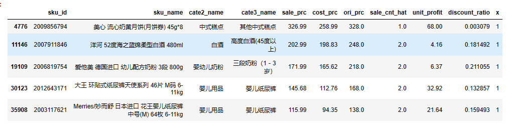
1）商品备选价格集合

# 制作每个sku的价格备选集合
prc_sale_cnt_sample = []
for row_id, sku in sku_cst_rhs_df.iterrows():
    for int_prc in range(int(sku.prc_lower), int(sku.prc_upper) + 1, 1):
        deci_prc_list = [0.58, 0.66, 0.68, 0.88, 0.98, 0.99]
        for deci_prc in deci_prc_list:
            prc = int_prc + deci_prc
            if sku.prc_lower < prc < sku.prc_upper:
                prc_sale_cnt_sample.append([sku.sku_id, sku.sku_name, sku.cate1_name, sku.cate2_name, sku.cate3_id, sku.cate3_name, sku.label, prc, sku.cost_prc_max, sku.ori_prc_max])
    # 添加成本价与原价(标签价)
    prc_sale_cnt_sample.append([sku.sku_id, sku.sku_name, sku.cate1_name, sku.cate2_name, sku.cate3_id, sku.cate3_name, sku.label, sku.prc_lower, sku.cost_prc_max, sku.ori_prc_max])
    prc_sale_cnt_sample.append([sku.sku_id, sku.sku_name, sku.cate1_name, sku.cate2_name, sku.cate3_id, sku.cate3_name, sku.label, sku.prc_upper, sku.cost_prc_max, sku.ori_prc_max])

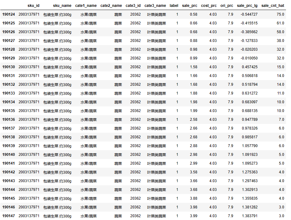
2）价格弹性预测

prc_sale_cnt_df['sale_prc_lg'] =  np.log(prc_sale_cnt_df['sale_prc'])
prc_sale_cnt_df['sale_cnt_hat'] = prc_sale_cnt_df.apply(func=predict_sku, axis=1)
prc_sale_cnt_df['sale_cnt_hat'] = prc_sale_cnt_df['sale_cnt_hat'].round(0)

3）ORTools 建模与 SCIP 求解

创建 solver

from ortools.linear_solver import pywraplp

mp_solver = pywraplp.Solver.CreateSolver('SCIP')
inf = mp_solver.infinity()
M = 1e7
tol = 1e-3
profit_ratio_lower = 0.2 + tol
profit_ratio_upper = 0.3 - tol
vegetable_min_discount_ratio = 0.3 + tol
fruit_min_discount_ratio = 0.2 + tol
pork_min_discount_ratio = 0.1 + tol
vegetable_c2 = '蔬菜'
fruit_c2 = '国产水果'
pork_c2 = '猪肉'

创建决策变量

sku_x_dict = defaultdict(list)
x_dict = {}
vegetable_x_dict = {}
fruit_x_dict = {}
pork_x_dict = {}

# 决策变量
for row_id, sku_prc in prc_sale_cnt_df.iterrows():
    x_key = '{}_{}'.format(sku_prc.sku_id, sku_prc.sale_prc)
    x = mp_solver.NumVar(0, 1, name=x_key)
    c = sku_prc.unit_profit * sku_prc.sale_cnt_hat
    x_dict[x_key] = (x, c, sku_prc)
    sku_x_dict[sku_prc.sku_id].append(x)
    if sku_prc.cate2_name == vegetable_c2:
        vegetable_x_dict[x_key] = (x, c, sku_prc)
    if sku_prc.cate2_name == fruit_c2:
        fruit_x_dict[x_key] = (x, c, sku_prc)
    if sku_prc.cate2_name == pork_c2:
        pork_x_dict[x_key] = (x, c, sku_prc)

# 松弛变量
profit_ratio_lower_slack = mp_solver.NumVar(0, inf, name='profit_ratio_lower_slack')
profit_ratio_upper_slack = mp_solver.NumVar(0, inf, name='profit_ratio_upper_slack')
vegetable_discount_ratio_lower_slack = mp_solver.NumVar(0, inf, name='vegetable_discount_ratio_lower_slack')
fruit_discount_ratio_lower_slack = mp_solver.NumVar(0, inf, name='fruit_discount_ratio_lower_slack')
pork_discount_ratio_lower_slack = mp_solver.NumVar(0, inf, name='pork_discount_ratio_lower_slack')

创建约束条件

st_dict = {}
st_list = []
# 每个sku只能选1个价格
for sku, xs in sku_x_dict.items():
    st = mp_solver.Constraint(1,1, str(sku))
    for x in xs:
        st.SetCoefficient(x, 1)
    st_dict[sku] = st
    st_list.append(st)

# 总利润率>=0.2
# sum(利润)  >= 0.2*sum(成本) ->  sum(利润) - 0.2*sum(成本) + slack >= 0
st = mp_solver.Constraint(0, inf, 'profit_ratio_lower_st')
for _, x_obj in x_dict.items():
    x, sku_prc = x_obj[0], x_obj[2]
    a = (sku_prc.unit_profit - profit_ratio_lower * sku_prc.cost_prc)* sku_prc.sale_cnt_hat
    st.SetCoefficient(x, a)
st.SetCoefficient(profit_ratio_lower_slack, 1)
st_dict['profit_ratio_lower_st'] = st
st_list.append(st)

# 总利润率<=0.3
# sum(利润) <= 0.3*sum(成本) ->  sum(利润) - 0.3*sum(成本) - slack <= 0
st = mp_solver.Constraint(-inf, 0, 'profit_ratio_upper_st')
for _, x_obj in x_dict.items():
    x, sku_prc = x_obj[0], x_obj[2]
    a = (sku_prc.unit_profit - profit_ratio_upper * sku_prc.cost_prc)* sku_prc.sale_cnt_hat
    st.SetCoefficient(x, a)
st.SetCoefficient(profit_ratio_upper_slack, -1)
st_dict['profit_ratio_upper_st'] = st
st_list.append(st)

# sum(折扣率) / sum(sku数) >= 最低折扣率  ->  sum(折扣率) -最低折扣率 * sum(sku数) + slack >= 0
# 蔬菜
st = mp_solver.Constraint(0, inf, 'vegetable_discount_ratio_lower_st')
for  _, x_obj in vegetable_x_dict.items():
    x, sku_prc = x_obj[0], x_obj[2]
    a = (sku_prc.discount_ratio - vegetable_min_discount_ratio * 1)
    st.SetCoefficient(x, a)
st.SetCoefficient(vegetable_discount_ratio_lower_slack, 1)
st_dict['vegetable_discount_ratio_lower_st'] = st
st_list.append(st)

# 国产水果
st = mp_solver.Constraint(0, inf, 'fruit_discount_ratio_lower_st')
for  _, x_obj in fruit_x_dict.items():
    x, sku_prc = x_obj[0], x_obj[2]
    a = (sku_prc.discount_ratio - fruit_min_discount_ratio * 1)
    st.SetCoefficient(x, a)
st.SetCoefficient(fruit_discount_ratio_lower_slack, 1)
st_dict['fruit_discount_ratio_lower_st'] = st
st_list.append(st)

# 猪肉
st = mp_solver.Constraint(0, inf, 'pork_discount_ratio_lower_st')
for  _, x_obj in pork_x_dict.items():
    x, sku_prc = x_obj[0], x_obj[2]
    a = (sku_prc.discount_ratio - pork_min_discount_ratio * 1)
    st.SetCoefficient(x, a)
st.SetCoefficient(pork_discount_ratio_lower_slack, 1)
st_dict['pork_discount_ratio_lower_st'] = st
st_list.append(st)

创建目标函数

# 目标
objective = mp_solver.Objective()
for _, x_obj in x_dict.items():
    x, c = x_obj[0], x_obj[1]
    objective.SetCoefficient(x, c)
objective.SetCoefficient(profit_ratio_lower_slack, -M)
objective.SetCoefficient(profit_ratio_upper_slack, -M)
objective.SetCoefficient(vegetable_discount_ratio_lower_slack, -M)
objective.SetCoefficient(fruit_discount_ratio_lower_slack, -M)
objective.SetCoefficient(pork_discount_ratio_lower_slack, -M)
objective.SetMaximization()

求解

 # 求解
f = open('./mp.lp', 'w')
f.write(mp_solver.ExportModelAsLpFormat(True))
# f.write(mp_solver.ExportModelAsLpFormat(False))
f.close()

mp_solver.EnableOutput() # 开启log
# mp_solver.SuppressOutput()
mp_solver.SetNumThreads(1)
mp_solver.SetTimeLimit(1000 * 1 * 300) # ms
param = pywraplp.MPSolverParameters()
param.PRESOLVE_ON = 1
param.RELATIVE_MIP_GAP = 0.0
status = mp_solver.Solve(param)

求解 log 如下：

presolving:
(round 1, fast)       18 del vars, 6 del conss, 0 add conss, 0 chg bounds, 0 chg sides, 0 chg coeffs, 0 upgd conss, 0 impls, 0 clqs
(round 2, fast)       18 del vars, 6 del conss, 0 add conss, 0 chg bounds, 12 chg sides, 0 chg coeffs, 0 upgd conss, 0 impls, 0 clqs
(round 3, fast)       218 del vars, 8 del conss, 0 add conss, 0 chg bounds, 12 chg sides, 0 chg coeffs, 0 upgd conss, 0 impls, 0 clqs
(round 4, exhaustive) 4178 del vars, 8 del conss, 0 add conss, 5 chg bounds, 12 chg sides, 0 chg coeffs, 0 upgd conss, 0 impls, 0 clqs
   Deactivated symmetry handling methods, since SCIP was built without symmetry detector (SYM=none).
presolving (5 rounds: 5 fast, 2 medium, 2 exhaustive):
 4178 deleted vars, 8 deleted constraints, 0 added constraints, 8 tightened bounds, 0 added holes, 12 changed sides, 0 changed coefficients
 0 implications, 0 cliques
presolved problem has 185999 variables (0 bin, 0 int, 0 impl, 185999 cont) and 3184 constraints
   3184 constraints of type <linear>
Presolving Time: 9.00

 time | node  | left  |LP iter|LP it/n|mem/heur|mdpt |vars |cons |rows |cuts |sepa|confs|strbr|  dualbound   | primalbound  |  gap   | compl.
*24.0s|     1 |     0 | 44153 |     - |    LP  |   0 | 185k|3184 |3184 |   0 |  0 |   0 |   0 | 3.694357e+04 | 3.694357e+04 |   0.00%| unknown
 24.0s|     1 |     0 | 44153 |     - |   851M |   0 | 185k|3184 |3184 |   0 |  0 |   0 |   0 | 3.694357e+04 | 3.694357e+04 |   0.00%| unknown

SCIP Status        : problem is solved [optimal solution found]
Solving Time (sec) : 24.00
Solving Nodes      : 1
Primal Bound       : +3.69435660720141e+04 (1 solutions)
Dual Bound         : +3.69435660720141e+04
Gap                : 0.00 %
[I 21:09:48.234 NotebookApp] Saving file at /4.model_algorithm_elasticity.ipynb
[I 21:11:47.859 NotebookApp] Saving file at /4.model_algorithm_elasticity.ipynb
[I 21:13:48.244 NotebookApp] Saving file at /4.model_algorithm_elasticity.ipynb
[I 21:15:44.505 NotebookApp] Saving file at /4.model_algorithm_elasticity.ipynb
[I 21:15:48.779 NotebookApp] Starting buffering for b14080f5-0663-41c6-b4f6-ac64dcade9f1:9a94821c2c27446a9b8551c893a4613f
[I 21:15:50.912 NotebookApp] Kernel restarted: b14080f5-0663-41c6-b4f6-ac64dcade9f1
[I 21:15:51.976 NotebookApp] Restoring connection for b14080f5-0663-41c6-b4f6-ac64dcade9f1:9a94821c2c27446a9b8551c893a4613f
[I 21:15:51.976 NotebookApp] Replaying 3 buffered messages
[I 21:17:54.218 NotebookApp] Saving file at /4.model_algorithm_elasticity.ipynb
presolving:
(round 1, fast)       18 del vars, 6 del conss, 0 add conss, 0 chg bounds, 0 chg sides, 0 chg coeffs, 0 upgd conss, 0 impls, 0 clqs
(round 2, fast)       18 del vars, 6 del conss, 0 add conss, 0 chg bounds, 12 chg sides, 0 chg coeffs, 0 upgd conss, 0 impls, 0 clqs
(round 3, fast)       218 del vars, 8 del conss, 0 add conss, 0 chg bounds, 12 chg sides, 0 chg coeffs, 0 upgd conss, 0 impls, 0 clqs
(round 4, exhaustive) 4178 del vars, 8 del conss, 0 add conss, 5 chg bounds, 12 chg sides, 0 chg coeffs, 0 upgd conss, 0 impls, 0 clqs
   Deactivated symmetry handling methods, since SCIP was built without symmetry detector (SYM=none).
presolving (5 rounds: 5 fast, 2 medium, 2 exhaustive):
 4178 deleted vars, 8 deleted constraints, 0 added constraints, 8 tightened bounds, 0 added holes, 12 changed sides, 0 changed coefficients
 0 implications, 0 cliques
presolved problem has 185999 variables (0 bin, 0 int, 0 impl, 185999 cont) and 3184 constraints
   3184 constraints of type <linear>
Presolving Time: 10.00

 time | node  | left  |LP iter|LP it/n|mem/heur|mdpt |vars |cons |rows |cuts |sepa|confs|strbr|  dualbound   | primalbound  |  gap   | compl.
*28.0s|     1 |     0 | 44372 |     - |    LP  |   0 | 185k|3184 |3184 |   0 |  0 |   0 |   0 | 3.694604e+04 | 3.694604e+04 |   0.00%| unknown
 28.0s|     1 |     0 | 44372 |     - |   851M |   0 | 185k|3184 |3184 |   0 |  0 |   0 |   0 | 3.694604e+04 | 3.694604e+04 |   0.00%| unknown

SCIP Status        : problem is solved [optimal solution found]
Solving Time (sec) : 28.00
Solving Nodes      : 1
Primal Bound       : +3.69460373439469e+04 (1 solutions)
Dual Bound         : +3.69460373439469e+04
Gap                : 0.00 %

4）结果统计

# 结果统计
sol_df['profit'] = sol_df['unit_profit'] * sol_df['sale_cnt_hat']
sol_df['cost'] = sol_df['cost_prc'] * sol_df['sale_cnt_hat']
sol_df['gmv'] = sol_df['sale_prc'] * sol_df['sale_cnt_hat']
sol_df['discount'] = sol_df['unit_profit'] * sol_df['sale_cnt_hat']
sol_df['ori_gmv'] = sol_df['ori_prc'] * sol_df['sale_cnt_hat']
profit = sol_df['profit'].sum()
cost = sol_df['cost'].sum()
gmv = sol_df['gmv'].sum()
discount_ratio = sol_df['discount_ratio'].mean()
vegetable_df = sol_df[(sol_df['cate2_name'] == vegetable_c2)]
fruit_df = sol_df[(sol_df['cate2_name'] == fruit_c2)]
pork_df = sol_df[(sol_df['cate2_name'] == pork_c2)]

print('最优解状态：', status)
print('总利润：',profit)
print('总成本：',cost)
print('总营收：',gmv)
print('总利润率:{}'.format(profit / cost))
print('总折扣率:{}'.format(discount_ratio))
print('蔬菜利润率:{}'.format(vegetable_df['profit'].sum() / vegetable_df['cost'].sum()))
print('蔬菜折扣率:{}'.format(vegetable_df['discount_ratio'].mean()))
print('国产水果利润率:{}'.format(fruit_df['profit'].sum() / fruit_df['cost'].sum()))
print('国产水果折扣率:{}'.format(fruit_df['discount_ratio'].mean()))
print('猪肉利润率:{}'.format(pork_df['profit'].sum() / pork_df['cost'].sum()))
print('猪肉折扣率:{}'.format(pork_df['discount_ratio'].mean()))

最优解状态： 0
总利润： 36880.27
总成本： 123319.58
总营收： 160199.84999999998
总利润率:0.2990625657336815
总折扣率:0.05771901890183243
蔬菜利润率:0.12843251752888687
蔬菜折扣率:0.2994485707115351
国产水果利润率:0.2352903707735693
国产水果折扣率:0.20145441470807798
猪肉利润率:0.2583410761044007
猪肉折扣率:0.14393190181238136

我们发现：模型求得了最优解，所有业务约束均被满足。 这说明了：精细化定价可以保证商家的利润，同时也能让消费者买到低价的商品，实现双赢。

当然，本篇只是讲解的最基础的版本，在实际业务落地时还需要考虑其他细化条件，如：连续多天定价、库存情况等。但整体求解框架不会有太大的改动。

04 本期小结

第一篇（业务问题拆解）：我们把一个实际的促销定价问题拆解成了一系列的数学问题。

第二篇（数据预处理生成）：我们选择了一份公开的促销定价数据集，将其加工成了可分析求解的数据。

第三篇（数据挖掘分析）：我们对数据进行了全方位的挖掘和分析，介绍了数据挖掘分析和可视化方法。

第四篇（价格弹性模型）：关于如何量化商品价格与销量的关系，我们详细介绍了baseline方案-价格弹性模型。

本篇（运筹决策模型）：我们详细介绍了如何价格弹性构建最终的定价运筹模型并调用开源求解工具ORTools求解。

05 下期预告

我们的系列推文的难度会逐系列递进。下期开始第二系列推送，会以选址和流量分配问题为切入，为大家呈现如何快速调用对比各大商业求解器（国产之光COPT、老牌巨头Gurobi/CPLEX、新锐之星MindOpt），重点在工程化实现层面有所拔高，敬请期待~~~

我们是**【运筹匠心】** ，咱们下期见~~~

参考文献

Hua J, Yan L, Xu H,et al. Markdowns in E-Commerce Fresh Retail: A Counterfactual Prediction and Multi-Period Optimization Approach[J]. arxiv, 2021.(https://arxiv.org/pdf/2105.08313.pdf)
Kui Zhao, Junhao Hua, Ling Yan, et al. A Unified Framework for Marketing Budget Allocation[J]. arxiv, 20.(https://arxiv.org/pdf/1902.01128.pdf)
用相关系数进行Kmeans聚类，利用利润率、打折率、销售额、毛利润得到商品价格弹性标签，建立价格折扣力度模型(https://blog.csdn.net/weixin_45934622/article/details/114382037)
2019全国大学生数学建模竞赛讲评：“薄利多销”分析(https://dxs.moe.gov.cn/zx/a/hd_sxjm_sxjmstjp_2019sxjmstjp/210604/1699445.shtml)
策略算法工程师之路-基于线性规划的简单价格优化模型(https://zhuanlan.zhihu.com/p/145192690)

运筹匠心

关注

18
点赞
踩
27

收藏

觉得还不错? 一键收藏
1
评论
【促销定价】背后的算法技术5-运筹决策模型

导读：本篇是【促销定价】系列5篇文章的最后一篇。用5篇文章，我们系统介绍了如何将一个实际的促销定问题转化为一个数学问题，并利用数据预处理与挖掘、统计学与机器学习、运筹优化等技术从 0-1 的解决该问题。帮助大家对定价算法落地应用有了一个基本的认识，为后续的深入学习奠定基础。作者 1：张哲铭，算法专家，某互联网大厂作者 2：向杜兵，算法专家，某制造业龙头明人不说暗话，【运筹匠心】想要大家的赞！赞！赞！。先赞后看，多多益善(*￣︶￣)~~~本期推文代码获取方式，将推文转发朋友圈获20赞，截图发后
复制链接

扫一扫