Coursera | Andrew Ng (01-week-2-2.9)—Logistic 回归中的梯度下降法

该系列仅在原课程基础上部分知识点添加个人学习笔记，或相关推导补充等。如有错误，还请批评指教。在学习了 Andrew Ng 课程的基础上，为了更方便的查阅复习，将其整理成文字。因本人一直在学习英语，所以该系列以英文为主，同时也建议读者以英文为主，中文辅助，以便后期进阶时，为学习相关领域的学术论文做铺垫。- ZJ

Coursera 课程 |deeplearning.ai |网易云课堂

---

转载请注明作者和出处：ZJ 微信公众号-「SelfImprovementLab」

知乎：https://zhuanlan.zhihu.com/c_147249273

CSDN：http://blog.csdn.net/JUNJUN_ZHAO/article/details/78913044

---

2.9 $logistic$ 回归中的梯度下降法
Logistic Regression Gradient Descent

(字幕来源：网易云课堂)

welcome back, in this video we’ll talk about how to compute derivatives for you,to implement gradient descent for $logistic$ regression.the key take aways will be what you need to implement that are the key equations you need,in order to implement gradient descent for $logistic$ regression.but in this video I want to do this computation,using the computation graph.I have to admit using the computation graph is a little bit of an overkill for deriving gradient descent for $logistic$ regression.but I want to start explaining things this way to get you familiar with these ideas.so that hopefully you’ll make a bit more sense when we talk about full fledged neural networks.

欢迎回来，在本节我们将讨论怎样计算偏导数，来实现 $logistic$ 回归的梯度下降法，它的核心关键点是 其中有几个重要的公式，用来实现 $logistic$ 回归的梯度下降法，但是在本节视频中 我将使用导数流程图，来计算梯度，必须承认，用导数流程图来计算 $logistic$ 回归的梯度下降 有点大材小用了，但是我认为以这种方式来讲解，可以更好地理解梯度下降，从而在讨论神经网络时，可以更深刻而全面地理解神经网络。

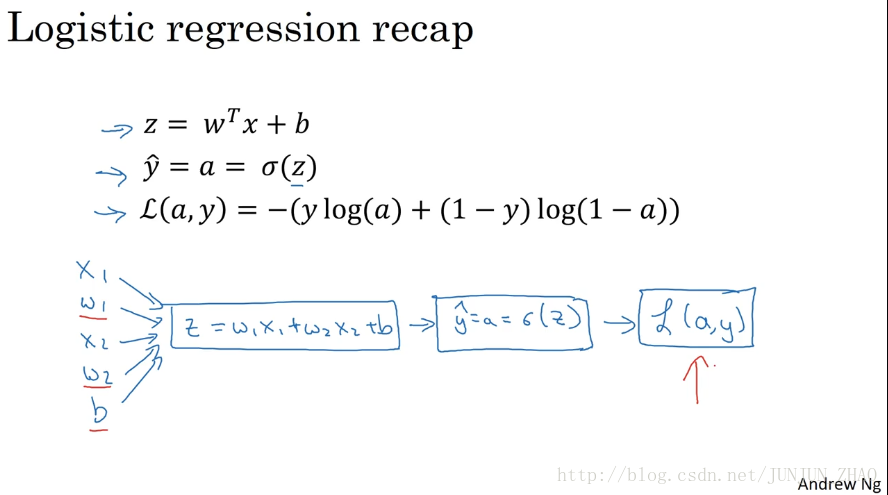
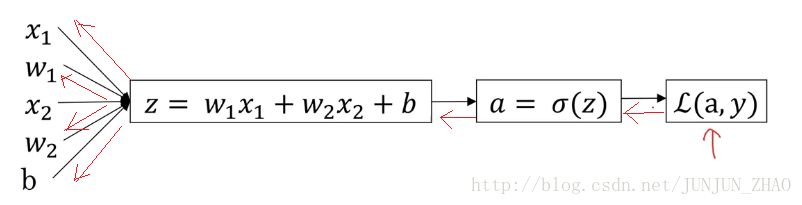
so let’s dive into gradient descent for $logistic$ regression to recap we had set up $logistic$ regression as follows your predictions y hat is defined as follows,where z is that and if we focus on just one example for now,then the loss or respect to that one example is defined as follows,where a is the output of the $logistic$ regression,and y is the ground truth label,so let’s write this out as a computation graph,and for this example let’s say we have only two features x1 and x2.so in order to compute z,we’ll need to input $w_1$ $w_2$ and b,in addition to the feature values x1 x2

接下来开始学习 $logistic$ 回归的梯度下降法， 回想一下 $logistic$ 回归的公式，$\hat{y}$ 定义如下 $\hat{y}$ 的定义是这样的，$z$ 则是这样 现在只考虑单个样本的情况，关于该样本的损失函数，定义如下，其中$a$是$logistic$回归的输出，$y$是样本的基本真值标签值，现在写出该样本的偏导数流程图，假设样本只有两个 特征$x1$和$x2$，为了计算$z$，我们需要输入参数$w_1$、$w_2$和$b$，还有样本特征值$x1$，$x2$。

so these things in a computation graph get used to compute z which is $w_1$ x1 plus $w_2$ x2 plus b.draw a rectangle box around that and then we compute y hat,or a equals Sigma of Z that’s the next step in a computation graph,and then finally we compute L(a,y),and I won’t copy the formula again,so in $logistic$ regression what we want to do,is to modify the parameters w and b,in order to reduce this loss,we’ve described before propagation steps,of how you actually compute the loss on a single training example.

因此用来计算$z$的 偏导数计算公式，$z$等于$w_1*x1+w_2*x2+b$，如图用矩形括起来了 然后计算$\hat{y}$，即$a$ 等于$sigma(z)$ 也就是偏导数流程图的下一步，最后计算$L(a,y)$，我不会再写出这个公式了，因此在$logistic$回归中 我们需要做的是，变换参数 $w$ 和 $b$ 的值，来最小化损失函数， 在前面我们已经前向传播步骤，在单个训练样本上计算损失函数。

now let’s talk about how you can go backwards to talk to compute the derivatives,here’s the cleaned up version of the diagram,because what we want to do is compute derivatives respect to this loss,the first thing we want to do we’re going backwards is to compute the derivative of this loss with respect to the script over there,with respect to this variable a,and so in the code,you know you just use da right to denote this variable,and it turns out that if you are familiar with calculus,you can show that this ends up being negative y over a,plus one minus y over one minus a,and the way you do that is you take the formula,for the loss and if you are familiar with calculus,you can compute the derivative with respect to the variable lowercase a and you get this formula.

现在让我们来 讨论怎样向后计算偏导数，这是整洁版本的图，要想计算损失函数L的导数，首先我们要，向前一步 先计算损失函数的导数，这里有个标记，关于变量$a$的导数，在代码中，你只需要使用$da$来表示这个变量，事实上 如果你熟悉微积分，这个结果是 $-y/a$，加上 $(1-y)/(1-a)$，损失函数导数的计算公式，就是这样 如果你熟悉微积分，你计算的关于变量$a$的导数，就是这个式子。

but if you’re not familiar of calculus,don’t worry about it,we’ll provide the derivative formulas you need,through out this course so if you are a expert in calculus,you’ll encourage you to look up the formula for the loss from their previous slide,and try to get director for respect to a using you know calculus,but if you don’t know enough calculus to do that,don’t worry about it,now having computed this quantity or da,the derivative of your final output variable respect to a,you can then go backwards and it turns out that you can show dz,which this is the Python code variable name,this is going to be you know the derivative of the loss,with respect to 关于 z or for L you can really write,the loss including a and y explicitly as parameters,or not right give either type of notation is equally acceptable they can show that,this is equal to a minus y,just a couple comments only for those of you did a experts in calculus.

如果你不熟悉微积分，也不必太担心，我们会列出本课程涉及的所有求导公式，因此 如果你非常熟悉微积分，我们鼓励你，通过上一张幻灯片中的损失函数公式，使用微积分 直接求出变量$a$的导数，如果你不太了解微积分，也不用太担心，现在计算出$da$，最终结果关于变量$a$的导数，现在可以再向后一步 计算$dz$，$dz$是代码中的变量名，$dz$是损失函数关于$z$的导数，对于$dL$，可以写成$dL(a,y)$，两种形式都可以，都是等价的，结果等于 $a-y$，给熟悉微积分的人解释一下。

if you’re not explain calculus,don’t worry about it,but it turns out that this right dL dz,this can be expressed as dL da times,da dz and it turns out that da dz,this turns out to be a times 1 minus a,and dL da we are previously worked out over here,and so if you take these two quantities dL da,which is this term together with da dz,which is this term and just take these two things,and multiply them you can show that you,the equation simplifies the a minus y,so that’s how you derive it,and this is really the chain rule that,and this is really the chain rule that.

如果你对微积分不熟悉，也不用担心，实际上 $dL/dz$，等于$(dL/da)$乘上，$da/dz$ 而$da/dz$，等于$a*(1-a)$，而$dL/da$ 在前面已经计算过了，因此将这两项$dL/da$，即这部分 和$da/dz$，这部分进行相乘，最终的公式，化简成 $(a-y$)，这个推导的过程，就是我之前提到过的“链式法则”。

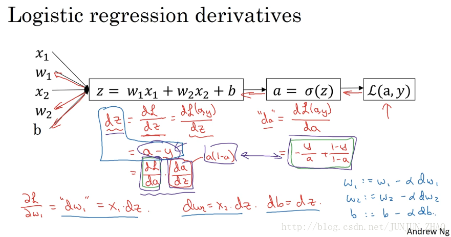
I briefly clue to you before ok,so feel free to go through that calculation yourself,if you are knowledgeable calculus,but if you aren’t all you need to know is that,you can compute dz as a minus y,and it already done the calculus for you,and then the final step in back propagation is to go back to compute how much you need to change w and b,so in particular you can show that the derivative respect to $w_1$,and will call this DW 1 that,this is equal to x1 times dz,and then similarly dw 2,which is how much you want to change $w_2$ is x2 times dz,and b excuse me $db$ is equal to dz.

如果你对微积分熟悉，放心地去计算，整个求导过程，如果不熟悉微积分,你只需要知道，$dz$ 等于 $(a-y)$，已经计算好了，现在向后传播的最后一步，特别地 关于$w_1$的导数 $dL/dw_1$，写成 $dw_1$，等于$x_1*dz$，同样地 $dw_2$，$w_2$的变化量 $dw_2$等于$x_2*dz$，$b$ 不好意思 应该是$db$等于dz。

so if you want to do gradient descents,with respect to just this one example,what you will do is the following,you would use this formula to compute dz,and then use these formulas to compute $dw_1$ $dw_2$,and $db$ and then you perform these,updates $w_1$ gets updated $w_1$ - learning rate alpha,rate alpha times $dw_1$ $w_2$ gets updated,similarly and B gets set as b - the learning rate times $db$,and so this will be one step of gradicent descent,with respect to a single example,so you’ve seen how to compute derivatives and implement gradient descent for $logistic$ regression with respect to a single training example.

因此关于单个样本的梯度下降法，你所需要做的就是这些事情，使用这个公式计算$dz$，使用这个计算$dw_1$、$dw_2$，还有$db$ 然后，更新$w_1$为 $w_1$减去学习率乘以$dw_1$，类似地 更新$w_2$，更新b 为b减去学习率乘以$db$，这就是单个样本实例的，一次梯度更新步骤，现在你已经知道了，怎样计算导数 并且实现了单个训练样本的，$logistic$回归的梯度下降法。

but to train $logistic$ regression model you have not just one training example,given entire training set of m training examples,so in the next video.let’s see how you can take these ideas and apply them,to learning not just from one example,but from an entire training set.

但是训练$logistic$回归模型，不仅仅只有一个训练样本，而是有 m 个训练样本的整个训练集，因此在下一节视频中，这些想法如何应用到，整个训练样本集中，而不仅仅只是单个样本上。

---

重点总结：

对单个样本而言，逻辑回归 Loss function 表达式：

$z= w^{T}x+b\\\hat y=a=\sigma(z)\\L(a, y)=-(y\log (a)+(1-y)\log(1-a))$

反向传播过程：（红色部分）

前面过程的 $da$、$dz$ 求导：

$da = \dfrac{\partial L}{\partial a}=-\dfrac{y}{a}+\dfrac{1-y}{1-a}\\dz = \dfrac{\partial L}{\partial z}=\dfrac{\partial L}{\partial a}\cdot\dfrac{\partial a}{\partial z}=(-\dfrac{y}{a}+\dfrac{1-y}{1-a})\cdot a(1-a)=a-y$

再对$w1、w2和b$进行求导：

$dw_{1} = \dfrac{\partial L}{\partial w_{1}}=\dfrac{\partial L}{\partial z}\cdot\dfrac{\partial z}{\partial w_{1}}=x_{1}\cdot dz=x_{1}(a-y)$

梯度下降法：

$w_{1}:=w_{1}-\alpha dw_{1}$

$w_{2}:=w_{2}-\alpha dw_{2}$

$b:=b-\alpha db$

参考文献：

[1]. 大树先生.吴恩达Coursera深度学习课程 DeepLearning.ai 提炼笔记（1-2）– 神经网络基础

---

PS: 欢迎扫码关注公众号：「SelfImprovementLab」！专注「深度学习」，「机器学习」，「人工智能」。以及 「早起」，「阅读」，「运动」，「英语 」「其他」不定期建群 打卡互助活动。