该系列仅在原课程基础上部分知识点添加个人学习笔记,或相关推导补充等。如有错误,还请批评指教。在学习了 Andrew Ng 课程的基础上,为了更方便的查阅复习,将其整理成文字。因本人一直在学习英语,所以该系列以英文为主,同时也建议读者以英文为主,中文辅助,以便后期进阶时,为学习相关领域的学术论文做铺垫。- ZJ
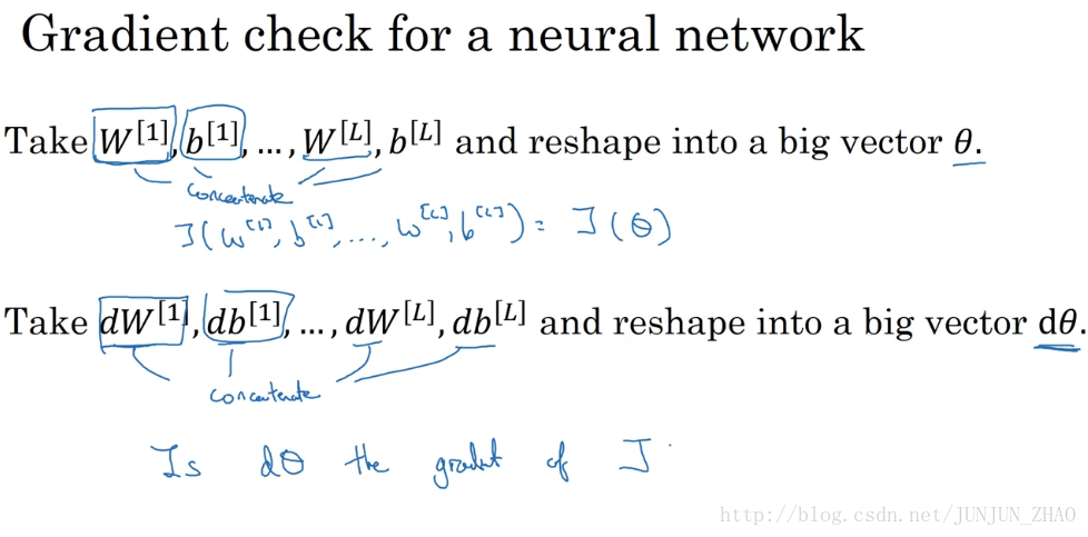
Gradient checking is a technique that’s helped me save tons of time, and helped me find bugs in my implementations of back propagation many times. Let’s see how you could use it too to debug, or to verify that your implementation and back props correct. So your new network will have some sort of parameters, W1, B1 and so on up to WL bL. So to implement gradient checking, the first thing you should do is take all your parameters and reshape them into a giant vector data. So what you should do is take W which is a matrix, and reshape it into a vector. You gotta take all of these Ws and reshape them into vectors, and then concatenate all of these things, so that you have a giant vector theta. Giant vector parameter as theta. So we say that the cos function J being a function of the Ws and Bs, You would now have the cost function J being just a function of theta.
梯度检验帮我节省了很多时间,也多次帮我发现 backprop 实施过程中的 bug,接下来 我们看看如何利用它来调试或检验 backpro的实施是否正确,假设你的网络中含有下列参数 W[1]和b[1]…. W[L]和b[L],为了执行梯度检验 首先要做的就是,把所有参数转换成一个巨大的向量数据,你要做的就是把矩阵 W 转换成一个向量,把所有 W 矩阵转换成向量之后,做连接运算 得到一个巨型向量θ,该向量表示为参数θ,代价函数J是所有 W 和 b 的函数,现在你得到了一个θ的代价函数J。
Next, with W and B ordered the same way, you can also take dW[1], db[1] and so on, and initiate them into big giant vector d theta of the same dimension as theta. So same as before, we shape dW[1] into the matrix, db[1] is already a vector. We shape dW[L],all of the dW’s which are matrices. Remember, dW1 has the same dimension as W1. db1 has the same dimension as b1. So the same sort of reshaping and concatenation operation, you can then reshape all of these derivatives into a giant vector d theta. Which has the same dimension as theta. So the question is,now,is the theta the gradient or the slope of the cos function J? So here’s how you implement gradient checking, and often abbreviate gradient checking to grad check.
接着 你得到与 W 和 b 顺序相同的数据,W[1]和db[1]…,用它们来初始化大向量dθ 它与θ具有相同维度,同样地 把dW[1]转换成矩阵 db[1]已经是一个向量了,直到把dW[L]转换成矩阵 这样所有的 dW 都已是矩阵,注意 dW[1]与 W1 具有相同维度,db1与 b1 具有相同维度,经过相同的转换和连接运算操作之后,你可以把所有导数转换成一个大向量dθ,它与θ具有相同维度,现在的问题是dθ,代价函数J的梯度或坡度有什么关系,这就是实施梯度检验的过程,英语里通常简称为“grad check”。
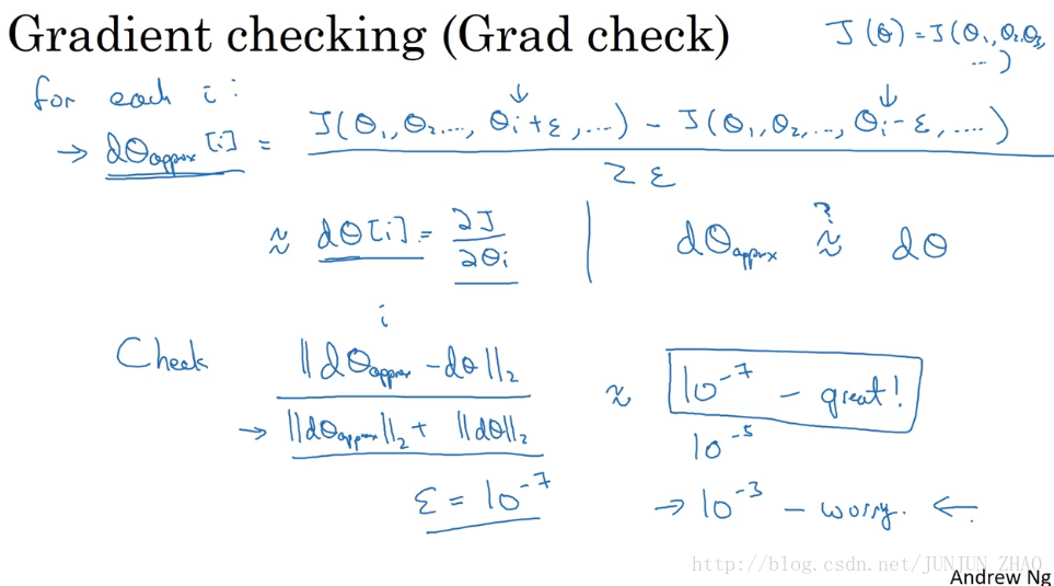
So first we remember that J Is now a function of the giant parameter, theta, right? So expands to j is a function of theta 1,theta 2, theta 3, and so on. Whatever’s the dimension of this giant parameter vector theta. So to implement grad check, what you’re going to do is implements a loop so that for each I, so for each component of theta, let’s compute D theta approx i to b. And I want to take a two sided difference. So I’ll take J of theta. Theta 1, theta 2, up to theta i. And we’re going to nudge theta i to add epsilon to this. So just increase theta i by epsilon, and keep everything else the same.And because we’re taking a two sided difference,we’re going to do the same on the other side with theta i, but now minus epsilon. And then all of the other elements of theta are left alone. And then we’ll take this, and we’ll divide it by 2 theta.And what we saw from the previous video is that this should be approximately equal to d theta [i], which is supposed to be the partial derivative of J or of respect to, I guess theta i, if d theta i is the derivative of the cost function J.So what you gonna do is you’re gonna compute to this for every value of i.And at the end, you now end up with two vectors.You end up with this d theta approx, and and this is going to be the same dimension as d theta.And both of these are in turn the same dimension as theta.And what you want to do is check if these vectors are approximately equal to each other.
首先 我们要清楚,J是超级参数θ的一个函数,你也可以将J函数展开为J(θ1,θ2,θ3....),不论超级参数向量θ的维度是多少,为了实施梯度检验 你要做的就是循环执行,从而对每个 i 也就是对每个θ组成元素,计算dθ[i]approx的值,我使用双边误差,也就是θ的J函数,J(θ1,θ2,….θi),θi调整为θi+ε,只对θi增加ε 其它项保持不变,因为我们使用的是双边误差,对另一边做同样的操作 只不过是减去 ε,θ其它项全都不保持不变,最后得到 J(θ1,θ2,….θi+ε,…)−J(θ1,θ2,….θi−ε,…)/2ε,从上节课中我们了解到,这个值应该逼近dθi,等于偏导数J比上θi 即,dθi是代价函数的偏导数,然后你需要对 i 的每个值都执行这个运算,最后得到两个向量,得到dθ的逼近值dθapprox,它与dθ具有相同维度,它们两个与θ具有相同维度,你要做的就是验证这些向量是否彼此接近。
So, in detail, well, how do you define whether or not two vectors are really reasonably close to each other? What I do is the following. I would compute the distance between these two vectors, d theta approx minus d theta, so just the o2 norm of this. Notice there’s no square on top, so this is the sum of squares of elements of the differences,and then you take a square root, as you get the Euclidean distance.And then just to normalize by the lengths of these vectors, divide by dθ approx plus dθ. Just take the Euclidean lengths of these vectors. And the row for the denominator is just in case any of these vectors are really small or really large, the denominator turns this formula into a ratio. So we implement this in practice,I use epsilon equals maybe 10 to the minus 7, so minus 7. And with this range of epsilon, if you find that this formula gives you a value like 10 to the minus 7 or smaller, then that’s great. It means that your derivative approximation is very likely correct. This is just a very small value. If it’s maybe on the range of 10 to the -5, I would take a careful look. Maybe this is okay. But I might double-check the components of this vector, and make sure that none of the components are too large. And if some of the components of this difference are very large, then maybe you have a bug somewhere.And if this formula on the left is on the other is -3, then I would worry, I would be much more concerned that maybe there’s a bug somewhere. But you should really be getting values much smaller than 10 minus 3, or if there is any bigger than 10 to minus 3, then I would be quite concerned. I would seriously worry about whether or not there might be a bug.And I would then, you should then look at the individual components of theta to see if there’s a specific value of i for which d theta approx i is very different from d theta i,and use that to try to track down whether or not some of your derivative computations might be incorrect.
And after some amounts of debugging, it finally, it ends up being this kind of very small value, then you probably have a correct implementation.So when implementing a neural network, what often happens is I’ll implement foreprop , implement backprop.And then I might find that this Grad check has a relatively big value. And then I will suspect that there must be a bug, go in debug, debug, debug.And after debugging for a while, If I find that it passes grad check with a small value,then you can be much more confident that it’s then correct. So you now know how gradient checking works. This has helped me find lots of bugs in my implementations of neural nets,and I hope it’ll help you too.In the next video, I want to share with you some tips or some notes on how to actually implement gradient checking. Let’s go onto the next video.
该系列仅在原课程基础上部分知识点添加个人学习笔记,或相关推导补充等。如有错误,还请批评指教。在学习了 Andrew Ng 课程的基础上,为了更方便的查阅复习,将其整理成文字。因本人一直在学习英语,所以该系列以英文为主,同时也建议读者以英文为主,中文辅助,以便后期进阶时,为学习相关领域的学术论文做铺垫。- ZJ Coursera 课程 |deeplearning.ai |网易云课堂


 88
88

 被折叠的 条评论
为什么被折叠?
被折叠的 条评论
为什么被折叠?
 到【灌水乐园】发言


