Coursera | Andrew Ng (02-week-1-1.10)—梯度消失与梯度爆炸

该系列仅在原课程基础上部分知识点添加个人学习笔记，或相关推导补充等。如有错误，还请批评指教。在学习了 Andrew Ng 课程的基础上，为了更方便的查阅复习，将其整理成文字。因本人一直在学习英语，所以该系列以英文为主，同时也建议读者以英文为主，中文辅助，以便后期进阶时，为学习相关领域的学术论文做铺垫。- ZJ

Coursera 课程 |deeplearning.ai |网易云课堂

---

转载请注明作者和出处：ZJ 微信公众号-「SelfImprovementLab」

知乎：https://zhuanlan.zhihu.com/c_147249273

CSDN：http://blog.csdn.net/junjun_zhao/article/details/79075145

---

1.10 vanishing/exploding gradients (梯度消失与梯度爆炸)

(字幕来源：网易云课堂)

One of the problems of training neural network, especially very deep neural networks, is data vanishing/exploding gradients. What that means is that when you’re training a very deep network, your derivatives or your slopes can sometimes get either very very big or very very small, maybe even exponentially small, and this makes training difficult. In this video, you see what this problem of exploding or vanishing gradients really means, as well as how you can use careful choices of the random weight initialization to significantly reduce this problem.

训练神经网络尤其是深度神经网络所面临的一个问题是，梯度消失或梯度爆炸，也就是说 当你训练深度网络时，导数或坡度有时会变得非常大，或非常小 甚至以指数方式变小， 这加大了训练的难度，这节课 你将会了解梯度消失或爆炸问题的真正含义，以及如何更明智地选择随机初始化权重，从而避免这个问题。

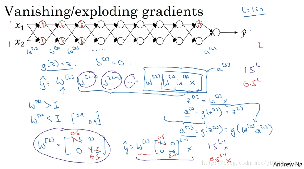
Let’s say you’re training a very deep neural network like this, to save space on the slide, I’ve drawn it as if you have only two hidden units per layer, but it could be more as well. But this neural network will have parameters $w^{[1]}$, $w^{[2]}$, $w^{[3]}$ and so on, up to $w^{[L]}$. For the sake of simplicity, let’s say we’re using an activation function $g(z)=z$,so linear activation function. And let’s ignore b, let’s say $b^{[L]}=0$. So in that case you can show that the output y will be $w^{[L]}$ times $w^{[L-1]}$ times $w^{[L-2]}$, dot, dot, dot down to the $w^{[3]}$, $w^{[2]}$, $w^{[1]}$ times x. But if you want to just check my math, $w^{[1]}$ times x is going to be $z^{[1]}$, right, because b is equal to zero. So $z^{[1]}$ is equal to, I guess, $w^{[1]}$ times x and then plus b which is zero. But then $a^{[1]}$ is equal to g of $z^{[1]}$. But because we use a linear activation function, this is just equal to $z^{[1]}$. So this first term $w^{[1]}$x is equal to $a^{[1]}$. And then by the reasoning you can figure out that $w^{[2]}$ times $w^{[1]}$ times x is equal to $a^{[2]}$, because that’s going to be g of $z^{[2]}$, is going to be g of $w^{[2]}$ times $a^{[1]}$which you can plug that in here. So this thing is going to be equal to $a^{[2]}$, and then this thing is going to be $a^{[3]}$, and so on until the protocol of all these matrices gives you $\hat{y}$, not y.

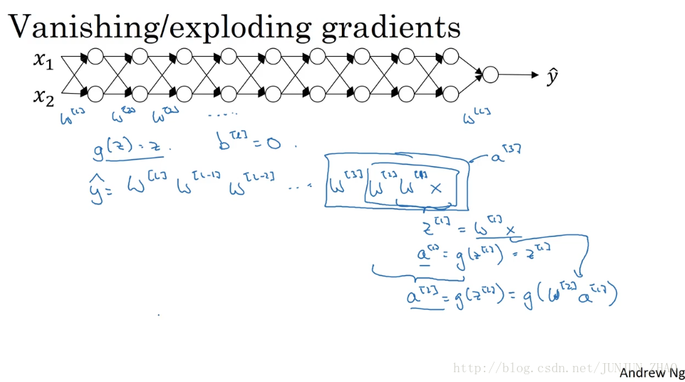
假设你正在训练这样一个极深的神经网络，为了节约幻灯片上的空间，我画的神经网络每层只有两个隐藏单元，但它可能含有更多，但这个神经网络会有参数$w^{[1]}$，$w^{[2]}$ $w^{[3]}$等等 直到$w^{[L]}$，为了简单起见，假设我们使用激活函数 $g(z)=z$，也就是线性激活函数，我们忽略 b 假设$b^{[L]}=0$，如果那样的话，输出$y=w^{[L]}*w^{[L-1]}*w^{[L-2]} .....w^{[3]}*w^{[2]}*w^{[1]}*x$，如果你想考验我的数学水平，$w^{[1]}*x=z^{[1]}$，因为 b 等于 0，所以我想，$z^{[1]}=w^{[1]}*x$ 因为b=0， $a^{[1]}=g(z^{[1]})$，因为我们使用了一个线性激活函数，它等于$z^{[1]}$，所以第一项$w^{[1]}*x$等于$a^{[1]}$，通过推理 你会得出$w^{[2]}*w^{[1]}*x=a^{[2]}$，因为$a^{[2]}=g(z^{[2]})$，还等于$g(w^{[2]}a^{[1]})$，可以用$w^{[1]}*x$替换$a^{[1]}$，所以这一项就等于$a^{[2]}$，这个就是$a^{[3]}$，所有这些矩阵数据传递的协议将给出$\hat{y}$而不是 y 的值。

Now, let’s say that each of you weight matrices $w^{[L]}$ is equal to… let’s say is just a little bit larger than one times the identity. So it’s 1.5_1.5_0_0. Technically, the last one has different dimensions, so maybe this is just the rest of these weight matrices. Then $\hat{y}$ will be, ignoring this last one with different dimension, will be this 1.5_0_0_1.5 matrix to the power of L minus 1 times X, because we assume that each one of these matrices is equal to this thing. It’s really 1.5 times the identity matrix, then you end up with this calculation. And so $\hat{Y}$ will be essentially 1.5 to the power of L, to the power of L minus 1 times X, and if L was large for very deep neural network, $\hat{Y}$ will be very large. In fact, this grows exponentially, it grows like 1.5 to the number of layers. And so if you have a very deep neural network, the value of y will explode.

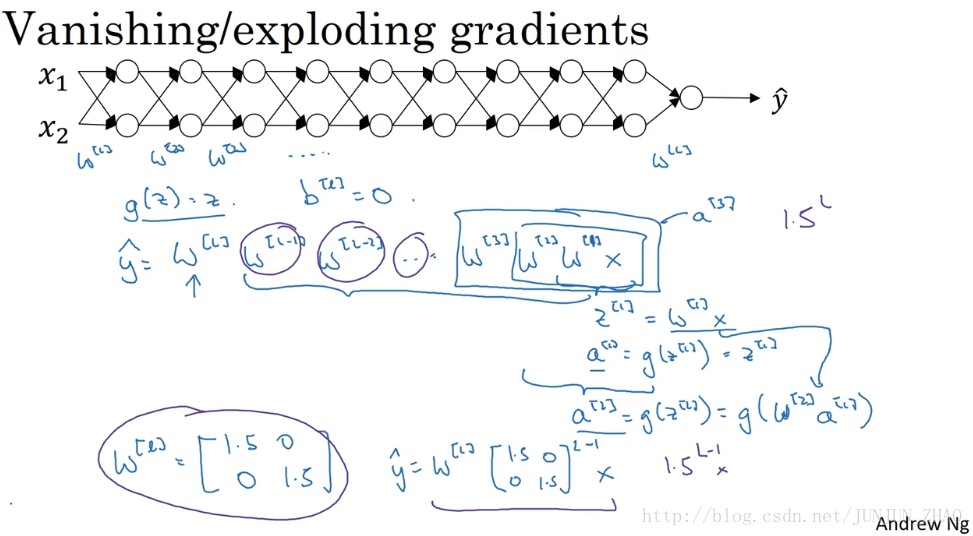
假设每个权重矩阵$w^{[L]}$等于…，假设它比 1 大一点，$w^{[L]}=[1.5,0,1.5,0]$，从技术上来讲 最后一项有不同维度，可能它就是余下的权重矩阵， $\hat{y}$等于，忽略最后这个不同维度的项，$\hat{y}$等于$w^{[1]}[1.5,0,0,1.5)]$ 的 L-1 次方乘以 x，因为我们假设所有矩阵都等于它，它是1.5倍的单位矩阵 最后的计算结果就是$\hat{y}$，$\hat{y}$也就等于$1.5^{(L-1)}$乘以 x。如果对于一个深度神经网络来说 L值较大，那么$\hat{y}$的值也会非常大，实际上它呈指数级增长的，它增长的比率是$1.5^{L}$，因此对于一个深度神经网络，y 的值将爆炸式增长。

Now, conversely, if we replace this with 0.5 , so something less than 1, then this becomes 0.5 to the power of L. This matrix becomes 0.5 to the L minus one times X, again ignoring $w^{[L]}$. And so each of your matrices are less than 1, then let’s say $x^{[1]}$, $x^{[2]}$ were one one, then the activations would be one half, one half, one fourth, one fourth, one eighth, one eighth, and so on, until this becomes 1 over 2 to the L. So the activation values will decrease exponentially as a function of the def, as a function of the number of layers L of the network. So in the very deep network, the activations end up decreasing exponentially.

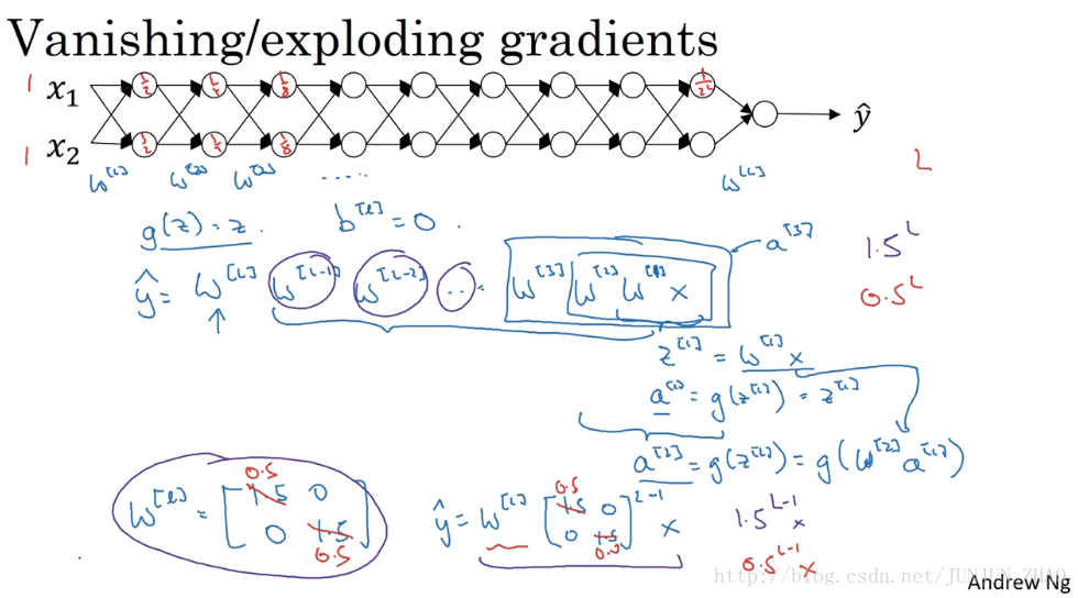
相反地 如果权重是 0.5 ，它比 1 小，这项也就变成了 $0.5^{L}$，矩阵$\hat{y}$=$w^{[1]}$乘以[ 0.5 ,0,0, 0.5 ]的 (L-1) 次方再乘以 x 再次忽略$w^{[L]}$，因此每个矩阵都小于 1，假设$x^{[1]}$ $x^{[2]}$都是 1，激活函数将变成 1/2 1/2，1/4 1/4 1/8 1/8 等，直到最后一项变成 1/2L，所以作为自定义函数 激活函数的值将以指数级下降，它是与网络层数量 L 相关的函数，在深度网络中 激活函数以指数级递减。

So the intuition I hope you can take away from this is that at the weights W, if they’re all, you know, just a little bit bigger than 1 or just a little bit bigger than the identity matrix, then with a very deep network, the activations can explode. And if W is you know just a little bit less than identity. So this maybe here’s 0.9, 0.9, then you have a very deep network, the activations will decrease exponentially. And even though I went through this argument in terms of activations increasing or decreasing exponentially as a function of L, a similar argument can be used to show that the derivatives or the gradients the computer is going to send will also increase exponentially or decrease exponentially as a function of the number of layers. With some of the modern neural networks, let’s say if L equals 150. Microsoft recently got great results with 152 layer neural network. But with such a deep neural network, if your activations or gradients increase or decrease exponentially as a function of L, then these values could get really big or really small. And this makes training difficult, especially if your gradients are exponentially smaller than L, then gradient descent will take tiny little steps. It will take a long time for gradient descent to learn anything.

我希望你得到的直观理解是，权重 W 只比 1 略大一点，或者说只比单位矩阵大一点，深度神经网络的激活函数将爆炸式增长，如果 W 比 1 略小一点，可能是 0.9,0.9，在深度神经网络中，激活函数将以指数级递减，虽然我只是论述了对 L 函数的激活函数，以指数级增长或下降，它也适用于与层数 L 相关的导数或梯度函数，也是呈指数增长，或呈指数递减，对于当前的神经网络 假设 L=150，最近 Microsoft 对 152 层神经网络的研究取得了很大进展，在这样一个深度神经网络中，如果作为 L 的函数的激活函数或梯度函数以指数级增长或递减，它们的值将会变得极大或极大，从而导致训练难度上升，尤其是梯度与 L 相差指数级，梯度下降算法的步长会非常非常小，梯度下降算法将花费很长时间来学习。

To summarize, you’ve seen how deep networks suffer from the problems of vanishing or exploding gradients. In fact, for a long time this problem was a huge barrier to training deep neural networks. It turns out there’s a partial solution that doesn’t completely solve this problem, but that helps a lot which is careful choice of how you initialize the weights. To see that, let’s go to the next video.

总结一下，今天我们讲了深度神经网络是如何产生梯度消失或爆炸问题的，实际上 在很长一段时间内 它曾是训练深度神经网络的阻力，虽然有一个不能彻底解决此问题的解决方案，但是已在如何选择初始化权重问题上提供了很多帮助，我们下节课继续讲。

---

重点总结：

梯度消失与梯度爆炸

如下图所示的神经网络结构，以两个输入为例：

这里我们首先假定$g(z)=z$，$b[l]=0$，所以对于目标输出有：

$\hat y = W^{[L]}W^{[L-1]}\cdots W^{[2]}W^{[1]}X$

• $W^{[l]}$ 的值大于1的情况：

  如：$W^{[l]}=\left[ \begin{array}{l} 1.5 & 0 \ 0 & 1.5\end{array} \right]$ ，那么最终，$\hat y = W^{[L]}\left[ \begin{array}{l} 1.5 & 0 \\\ 0 & 1.5\end{array} \right]^{L-1}X$ ，激活函数的值将以指数级递增；

• $W^{[l]}$ 的值小于1的情况：

  如：$W^{[l]}=\left[ \begin{array}{l} 0.5 & 0 \ 0 & 0.5\end{array} \right]$ ，那么最终，$\hat y = W^{[L]}\left[ \begin{array}{l} 0.5 & 0 \\\ 0 & 0.5\end{array} \right]^{L-1}X$ ,激活函数的值将以指数级递减。

上面的情况对于导数也是同样的道理，所以在计算梯度时，根据情况的不同，梯度函数会以指数级递增或者递减，导致训练导数难度上升，梯度下降算法的步长会变得非常非常小，需要训练的时间将会非常长。

在梯度函数上出现的以指数级递增或者递减的情况就分别称为梯度爆炸或者梯度消失。

参考文献：

[1]. 大树先生.吴恩达Coursera深度学习课程 DeepLearning.ai 提炼笔记（2-1）– 深度学习的实践方面

---

PS: 欢迎扫码关注公众号：「SelfImprovementLab」！专注「深度学习」，「机器学习」，「人工智能」。以及 「早起」，「阅读」，「运动」，「英语 」「其他」不定期建群 打卡互助活动。