全网最详细的Transformer的源码解读

最新推荐文章于 2024-03-02 22:20:51 发布

熊思健WHUT

最新推荐文章于 2024-03-02 22:20:51 发布

阅读量964

点赞数 2

文章标签： transformer 深度学习自然语言处理

本文链接：https://blog.csdn.net/JamesX666/article/details/126454270

版权

输入部分实现

文本嵌入层

# 导入必备的工具包
import torch

# 预定义的网络层torch.nn, 工具开发者已经帮助我们开发好的一些常用层, 
# 比如，卷积层, lstm层, embedding层等, 不需要我们再重新造轮子.
import torch.nn as nn

# 数学计算工具包
import math

# torch中变量封装函数Variable. 扩展资料: https://www.jb51.net/article/177996.htm
from torch.autograd import Variable

# 定义Embeddings类来实现文本嵌入层，这里s说明代表两个一模一样的嵌入层, 他们共享参数.
# 该类继承nn.Module, 这样就有标准层的一些功能, 这里我们也可以理解为一种模式, 我们自己实现的所有层都会这样去写.
class Embeddings(nn.Module):
    def __init__(self, d_model, vocab):
        """类的初始化函数, 有两个参数, d_model: 指词嵌入的维度, vocab: 指词表的大小."""
        # 接着就是使用super的方式指明继承nn.Module的初始化函数, 我们自己实现的所有层都会这样去写.
        super(Embeddings, self).__init__()
        # 之后就是调用nn中的预定义层Embedding, 获得一个词嵌入对象self.lut
        self.lut = nn.Embedding(vocab, d_model)
        # 最后就是将d_model传入类中
        self.d_model = d_model

    def forward(self, x):
        """可以将其理解为该层的前向传播逻辑，所有层中都会有此函数
           当传给该类的实例化对象参数时, 自动调用该类函数
           参数x: 因为Embedding层是首层, 所以代表输入给模型的文本通过词汇映射后的张量"""

        # 将x传给self.lut并与根号下self.d_model相乘作为结果返回
        return self.lut(x) * math.sqrt(self.d_model)

# nn.Embedding演示
embedding = nn.Embedding(10, 3)
input = torch.LongTensor([[1,2,4,5],[4,3,2,9]])
embedding(input)

tensor([[[-0.3101,  0.4961, -0.1494],
         [-0.2178, -0.3668,  0.9646],
         [ 1.2691, -0.6192, -0.0714],
         [-0.3463, -1.7143, -0.6863]],

        [[ 1.2691, -0.6192, -0.0714],
         [-0.1814,  0.3438, -1.6297],
         [-0.2178, -0.3668,  0.9646],
         [-1.3767,  0.2328,  0.6870]]], grad_fn=<EmbeddingBackward>)


embedding = nn.Embedding(10, 3, padding_idx=0)
input = torch.LongTensor([[0,2,0,5]])
embedding(input)

tensor([[[ 0.0000,  0.0000,  0.0000],
         [ 0.7241,  0.0428, -1.0146],
         [ 0.0000,  0.0000,  0.0000],
         [-1.2611,  0.8732,  0.3194]]], grad_fn=<EmbeddingBackward>)


# embedding演示
# 8代表的是词表的大小, 也就是只能编码0-7
# 如果是10， 代表只能编码0-9  这里有11出现所以尚明embedding的时候要写成12
# embedding = nn.Embedding(10, 4)
# input = torch.LongTensor([[1, 2, 3, 4], [4, 9, 2, 1]])
# print('----:', embedding(input))


# # padding_idx代表的意思就是和给定的值相同， 那么就用0填充， 比如idx=2那么第二行就是0
embedding = nn.Embedding(10, 3, padding_idx=2)
input = torch.LongTensor([[0,2,0,5]])
print(embedding(input))
tensor([[[ 0.7556,  1.2365, -0.1391],
         [ 0.0000,  0.0000,  0.0000],
         [ 0.7556,  1.2365, -0.1391],
         [-1.0002, -0.9913,  0.3016]]], grad_fn=<EmbeddingBackward>)


# 调用验证
# 词嵌入维度是512维
d_model = 512

# 词表大小是1000
vocab = 1000

# 输入x是一个使用Variable封装的长整型张量, 形状是2 x 4
# 关于Variable的使用：https://blog.csdn.net/u012370185/article/details/94391428
x = Variable(torch.LongTensor([[100,2,421,508],[491,998,1,221]]))

emb = Embeddings(d_model, vocab)
embr = emb(x)
print("embr:", embr)
print('embrshape', embr.shape)

embr: tensor([[[ 40.2344, -21.8559,  -3.0786,  ..., -39.4450,   6.3441, -18.0641],
         [  1.8564,   3.9727, -21.6685,  ...,  19.8701,  43.0585,  -2.7499],
         [-24.5998, -13.8384, -25.0284,  ...,  11.5420,   9.2373, -21.2582],
         [ 24.9655, -40.3250,   7.2429,  ..., -10.7791,  40.0044,   3.1575]],

        [[ 12.8280,  -5.5107,  10.4777,  ..., -11.7140,  -1.3078, -14.4176],
         [ 18.9400,  26.3958,  14.5878,  ...,  -3.0378,  -4.1521, -24.7141],
         [ -7.3845,  -4.6254, -52.0248,  ...,  13.4017,  14.4252, -18.3516],
         [-10.4541,  26.8224,   3.8177,  ...,  -6.6592,   8.2692, -16.1433]]],
       grad_fn=<MulBackward0>)
embrshape torch.Size([2, 4, 512])

位置编码器


# 定义位置编码器类, 我们同样把它看做一个层, 因此会继承nn.Module    
class PositionalEncoding(nn.Module):
    def __init__(self, d_model, dropout, max_len=5000):
        """位置编码器类的初始化函数, 共有三个参数, 分别是d_model: 词嵌入维度,dropout: 置0比率, max_len: 每个句子的最大长度"""
        super(PositionalEncoding, self).__init__()

        # 实例化nn中预定义的Dropout层, 并将dropout传入其中, 获得对象self.dropout
        self.dropout = nn.Dropout(p=dropout)

        # 初始化一个位置编码矩阵, 它是一个0阵，矩阵的大小是max_len x d_model.
        pe = torch.zeros(max_len, d_model)

        # 初始化一个绝对位置矩阵, 在我们这里，词汇的绝对位置就是用它的索引去表示. 
        # 所以我们首先使用arange方法获得一个连续自然数向量，然后再使用unsqueeze方法拓展向量维度使其成为矩阵， 
        # 又因为参数传的是1，代表矩阵拓展的位置，会使向量变成一个max_len x 1 的矩阵， 
        position = torch.arange(0, max_len).unsqueeze(1)

        # 绝对位置矩阵初始化之后，接下来就是考虑如何将这些位置信息加入到位置编码矩阵中，
        # 最简单思路就是先将max_len x 1的绝对位置矩阵， 变换成max_len x d_model形状，然后覆盖原来的初始位置编码矩阵即可， 
        # 要做这种矩阵变换，就需要一个1xd_model形状的变换矩阵div_term，我们对这个变换矩阵的要求除了形状外，还希望它能够将自然数的绝对位置编码缩放成足够小的数字，有助于在之后的梯度下降过程中更快的收敛.  这样我们就可以开始初始化这个变换矩阵了.
        # 首先使用arange获得一个自然数矩阵， 我们这里并没有按照预计的一样初始化一个1xd_model的矩阵， 而是有了一个跳跃，只初始化了一半即1xd_model/2 的矩阵。 为什么是一半呢，其实这里并不是真正意义上的初始化了一半的矩阵
        # 我们可以把它看作是初始化了两次，而每次初始化的变换矩阵会做不同的处理，第一次初始化的变换矩阵分布在正弦波上， 第二次初始化的变换矩阵分布在余弦波上，并把这两个矩阵分别填充在位置编码矩阵的偶数和奇数位置上，组成最终的位置编码矩阵.
        div_term = torch.exp(torch.arange(0, d_model, 2) *(math.log(10000.0) / d_model))
        pe[:, 0::2] = torch.sin(position * div_term)
        pe[:, 1::2] = torch.cos(position * div_term)

        # 这样我们就得到了位置编码矩阵pe, pe现在还只是一个二维矩阵，要想和embedding的输出（一个三维张量）相加，
        # 就必须拓展一个维度，所以这里使用unsqueeze拓展维度.
        pe = pe.unsqueeze(0)

        # 最后把pe位置编码矩阵注册成模型的buffer，什么是buffer呢，
        # 我们把它认为是对模型效果有帮助的，但是却不是模型结构中超参数或者参数，不需要随着优化步骤进行更新的增益对象. 
        # 注册之后我们就可以在模型保存后重加载时和模型结构与参数一同被加载.
        '''
        向模块添加持久缓冲区。
        这通常用于注册不应被视为模型参数的缓冲区。例如，pe不是一个参数，而是持久状态的一部分。
        缓冲区可以使用给定的名称作为属性访问。
        
        说明：
        应该就是在内存中定义一个常量，同时，模型保存和加载的时候可以写入和读出
        '''
        self.register_buffer('pe', pe)

    def forward(self, x):
        """forward函数的参数是x, 表示文本序列的词嵌入表示"""
        # 在相加之前我们对pe做一些适配工作， 将这个三维张量的第二维也就是句子最大长度的那一维将切片到与输入的x的第二维相同即x.size(1)，
        # 因为我们默认max_len为5000一般来讲实在太大了，很难有一条句子包含5000个词汇，所以要进行与输入张量的适配. 
        # 最后使用Variable进行封装，使其与x的样式相同，但是它是不需要进行梯度求解的，因此把requires_grad设置成false.
        print("=====", x.size())
        print("-=-=-=", x.size(1))
        print('peshape', self.pe.shape)
        print('pe_shape', self.pe[:, :x.size(1)].shape)
        x = x + Variable(self.pe[:, :x.size(1)], 
                         requires_grad=False)
        # 最后使用self.dropout对象进行'丢弃'操作, 并返回结果.
        return self.dropout(x)


# nn.Dropout演示
m = nn.Dropout(p=0.2)
input = torch.randn(4, 5)
output = m(input)
output
tensor([[ 0.1332,  1.6906,  2.0688,  0.0000, -0.0000],
        [-1.3093,  0.0000, -0.6924, -3.4059,  1.3496],
        [-0.5986, -0.4578,  0.9641, -1.6181, -1.2664],
        [ 0.8293,  0.0834,  0.9775,  0.2243, -1.3071]])

# torch.unsqueeze演示
x = torch.tensor([1, 2, 3, 4])
torch.unsqueeze(x, 0)
tensor([[1, 2, 3, 4]])

torch.unsqueeze(x, 1)
tensor([[1],
        [2],
        [3],
        [4]])


 x = torch.tensor([1, 2, 3, 4])
# 在行的维度添加， 三维度添加之后， 形状是一样的
# print(torch.unsqueeze(x, 0))
# print(torch.unsqueeze(x, 0).shape)
# print(x.unsqueeze(0))
# print(x.unsqueeze(1))
# 在列的维度添加  三纬度添加之后， 不管是写1还是0， 形状都是一样的
# print(torch.unsqueeze(x, 1))
# print(torch.unsqueeze(x, 1).shape)

# 调用验证
# 词嵌入维度是512维
d_model = 512

# 置0比率为0.1
dropout = 0.1

# 句子最大长度
max_len=60

# 输入x是Embedding层的输出的张量, 形状是2 x 4 x 512
x = embr

pe = PositionalEncoding(d_model, dropout, max_len)
pe_result = pe(x)
print("pe_result:", pe_result)


===== torch.Size([2, 4, 512])
-=-=-= 4
peshape torch.Size([1, 60, 512])
pe_shape torch.Size([1, 4, 512])
pe_result: tensor([[[ 44.7049, -23.1732,  -3.4207,  ...,  -0.0000,   7.0490, -18.9601],
         [  2.9977,   5.0144, -23.1629,  ...,  23.1890,  47.8429,  -1.9443],
         [-26.3228, -15.8384, -26.7689,  ...,  13.9356,  10.2639, -22.5091],
         [ 27.8963, -45.9055,   8.3199,  ..., -10.8656,  44.4497,   4.6194]],

        [[ 14.2534,  -5.0119,  11.6419,  ..., -11.9045,  -1.4532, -14.9084],
         [ 21.9794,   0.0000,  17.1219,  ...,  -2.2642,  -4.6133, -26.3490],
         [ -7.1947,  -5.6017, -56.7649,  ...,   0.0000,  16.0282, -19.2796],
         [-11.4589,  28.7027,   4.5142,  ...,  -6.2880,   9.1883, -16.8259]]],
       grad_fn=<MulBackward0>)

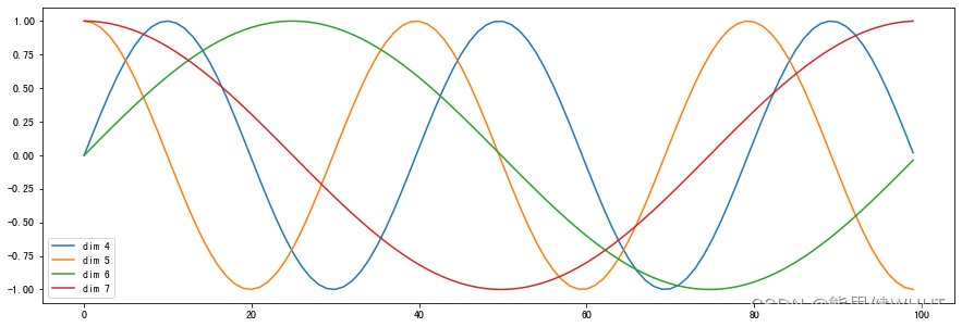
绘制词汇向量中特征的分布曲线


```python
import matplotlib.pyplot as plt
import numpy as np

# 创建一张15 x 5大小的画布
plt.figure(figsize=(15, 5))

# 实例化PositionalEncoding类得到pe对象, 输入参数是20和0
pe = PositionalEncoding(20, 0)

# 然后向pe传入被Variable封装的tensor, 这样pe会直接执行forward函数, 
# 且这个tensor里的数值都是0, 被处理后相当于位置编码张量
y = pe(Variable(torch.zeros(1, 100, 20)))

# 然后定义画布的横纵坐标, 横坐标到100的长度, 纵坐标是某一个词汇中的某维特征在不同长度下对应的值
# 因为总共有20维之多, 我们这里只查看4，5，6，7维的值.
plt.plot(np.arange(100), y[0, :, 4:8].data.numpy())

# 在画布上填写维度提示信息
plt.legend(["dim %d"%p for p in [4,5,6,7]])
plt.show()

===== torch.Size([1, 100, 20])
-=-=-= 100
peshape torch.Size([1, 5000, 20])
pe_shape torch.Size([1, 100, 20])

![Position Encoding](https://img-blog.csdnimg.cn/8def9ea4513247ff8fa2f5783e0a330a.png)


##  编码器部分实现
# 掩码张量

```python
def subsequent_mask(size):
    """生成向后遮掩的掩码张量, 参数size是掩码张量最后两个维度的大小, 它的最后两维形成一个方阵"""
    # 在函数中, 首先定义掩码张量的形状
    attn_shape = (1, size, size)

    # 然后使用np.ones方法向这个形状中添加1元素,形成上三角阵, 最后为了节约空间, 
    # 再使其中的数据类型变为无符号8位整形unit8 
    subsequent_mask = np.triu(np.ones(attn_shape), k=1).astype('uint8')

    # 最后将numpy类型转化为torch中的tensor, 内部做一个1 - 的操作, 
    # 在这个其实是做了一个三角阵的反转, subsequent_mask中的每个元素都会被1减, 
    # 如果是0, subsequent_mask中的该位置由0变成1
    # 如果是1, subsequent_mask中的该位置由1变成0 
    return torch.from_numpy(1 - subsequent_mask)

# def triu（m, k）
# m：表示一个矩阵
# K：表示对角线的起始位置（k取值默认为0）
# return: 返回函数的上三角矩阵

# np.triu演示
np.triu([[1,2,3],[4,5,6],[7,8,9],[10,11,12]], k=-1)
array([[ 1,  2,  3],
       [ 4,  5,  6],
       [ 0,  8,  9],
       [ 0,  0, 12]])

np.triu([[1,2,3],[4,5,6],[7,8,9],[10,11,12]], k=0)
array([[1, 2, 3],
       [0, 5, 6],
       [0, 0, 9],
       [0, 0, 0]])

np.triu([[1,2,3],[4,5,6],[7,8,9],[10,11,12]], k=1)
array([[1, 2, 3],
       [0, 5, 6],
       [0, 0, 9],
       [0, 0, 0]])

# 调用验证
# 生成的掩码张量的最后两维的大小
size = 5
sm = subsequent_mask(size)
print("sm:", sm)
sm: tensor([[[1, 0, 0, 0, 0],
         [1, 1, 0, 0, 0],
         [1, 1, 1, 0, 0],
         [1, 1, 1, 1, 0],
         [1, 1, 1, 1, 1]]], dtype=torch.uint8)

#掩码张量的可视化
plt.figure(figsize=(5,5))
plt.imshow(subsequent_mask(20)[0])
plt.show()

注意力机制

import torch.nn.functional as F
def attention(query, key, value, mask=None, dropout=None):
    """注意力机制的实现, 输入分别是query, key, value, mask: 掩码张量, 
       dropout是nn.Dropout层的实例化对象, 默认为None"""
    # 在函数中, 首先取query的最后一维的大小, 一般情况下就等同于我们的词嵌入维度, 命名为d_k
    d_k = query.size(-1)
    # print('query===', query)
#   # print('queryshape===', query.shape)
    #queryshape=== torch.Size([2, 4, 512]) 2表示有2个样本， 4表示每个样本中四个词，512表示把每个词映射到512维度上(可以理解为512个特征)
    # print('keyshape====', key.shape) # keyshape==== torch.Size([2, 4, 512])
#   # print('keytranspose====', key.transpose(-2, -1).shape) # keytranspose==== torch.Size([2, 512, 4])
    # 按照注意力公式, 将query与key的转置相乘, 这里面key是将最后两个维度进行转置, 再除以缩放系数根号下d_k, 这种计算方法也称为缩放点积注意力计算.
    # 得到注意力得分张量scores
    scores = torch.matmul(query, key.transpose(-2, -1)) / math.sqrt(d_k)

    # 接着判断是否使用掩码张量
    if mask is not None:
        # 使用tensor的masked_fill方法, 将掩码张量和scores张量每个位置一一比较, 如果掩码张量处为0
        # 则对应的scores张量用-1e9这个值来替换, 如下演示
        scores = scores.masked_fill(mask == 0, -1e9)

    # 对scores的最后一维进行softmax操作, 使用F.softmax方法, 第一个参数是softmax对象, 第二个是目标维度.
    # 这样获得最终的注意力张量
    p_attn = F.softmax(scores, dim = -1)

    # 之后判断是否使用dropout进行随机置0
    if dropout is not None:
        # 将p_attn传入dropout对象中进行'丢弃'处理
        p_attn = dropout(p_attn)

    # 最后, 根据公式将p_attn与value张量相乘获得最终的query注意力表示, 同时返回注意力张量
    return torch.matmul(p_attn, value), p_attn

# tensor.masked_fill演示
input = Variable(torch.randn(5, 5))
input
tensor([[ 2.2359,  1.9652,  1.8737,  1.6435, -0.6214],
        [ 0.5453, -0.3968, -0.3690,  1.3170, -0.2986],
        [-0.5605,  0.2373, -1.2774, -1.0373, -1.5568],
        [ 0.8109,  1.8287, -2.8008, -0.1955,  1.1374],
        [-0.9810,  0.6821,  0.2788,  1.4857, -2.5654]])

mask = Variable(torch.zeros(5, 5))
mask
tensor([[0., 0., 0., 0., 0.],
        [0., 0., 0., 0., 0.],
        [0., 0., 0., 0., 0.],
        [0., 0., 0., 0., 0.],
        [0., 0., 0., 0., 0.]])

input.masked_fill(mask == 0, -1e9)
tensor([[-1.0000e+09, -1.0000e+09, -1.0000e+09, -1.0000e+09, -1.0000e+09],
        [-1.0000e+09, -1.0000e+09, -1.0000e+09, -1.0000e+09, -1.0000e+09],
        [-1.0000e+09, -1.0000e+09, -1.0000e+09, -1.0000e+09, -1.0000e+09],
        [-1.0000e+09, -1.0000e+09, -1.0000e+09, -1.0000e+09, -1.0000e+09],
        [-1.0000e+09, -1.0000e+09, -1.0000e+09, -1.0000e+09, -1.0000e+09]])

# 调用验证
# 我们令输入的query, key, value都相同, 位置编码的输出
query = key = value = pe_result
attn, p_attn = attention(query, key, value)
print("attn:", attn)
print("p_attn:", p_attn)

attn: tensor([[[ 44.7049, -23.1732,  -3.4207,  ...,   0.0000,   7.0490, -18.9601],
         [  2.9977,   5.0144, -23.1629,  ...,  23.1890,  47.8429,  -1.9443],
         [-26.3228, -15.8384, -26.7689,  ...,  13.9356,  10.2639, -22.5091],
         [ 27.8963, -45.9055,   8.3199,  ..., -10.8656,  44.4497,   4.6194]],

        [[ 14.2534,  -5.0119,  11.6419,  ..., -11.9045,  -1.4532, -14.9084],
         [ 21.9794,   0.0000,  17.1219,  ...,  -2.2642,  -4.6133, -26.3490],
         [ -7.1947,  -5.6017, -56.7649,  ...,   0.0000,  16.0282, -19.2796],
         [-11.4589,  28.7027,   4.5142,  ...,  -6.2880,   9.1883, -16.8259]]],
       grad_fn=<UnsafeViewBackward>)
p_attn: tensor([[[1., 0., 0., 0.],
         [0., 1., 0., 0.],
         [0., 0., 1., 0.],
         [0., 0., 0., 1.]],

        [[1., 0., 0., 0.],
         [0., 1., 0., 0.],
         [0., 0., 1., 0.],
         [0., 0., 0., 1.]]], grad_fn=<SoftmaxBackward>)

带有mask的输入参数
query = key = value = pe_result

# 令mask为一个2x4x4的零张量
mask = Variable(torch.zeros(2, 4, 4))
attn, p_attn = attention(query, key, value, mask=mask)
print("attn:", attn)
print("p_attn:", p_attn)


attn: tensor([[[ 12.3190, -19.9757, -11.2581,  ...,   6.5647,  27.4014,  -9.6985],
         [ 12.3190, -19.9757, -11.2581,  ...,   6.5647,  27.4014,  -9.6985],
         [ 12.3190, -19.9757, -11.2581,  ...,   6.5647,  27.4014,  -9.6985],
         [ 12.3190, -19.9757, -11.2581,  ...,   6.5647,  27.4014,  -9.6985]],

        [[  4.3948,   4.5223,  -5.8717,  ...,  -5.1142,   4.7875, -19.3407],
         [  4.3948,   4.5223,  -5.8717,  ...,  -5.1142,   4.7875, -19.3407],
         [  4.3948,   4.5223,  -5.8717,  ...,  -5.1142,   4.7875, -19.3407],
         [  4.3948,   4.5223,  -5.8717,  ...,  -5.1142,   4.7875, -19.3407]]],
       grad_fn=<UnsafeViewBackward>)
p_attn: tensor([[[0.2500, 0.2500, 0.2500, 0.2500],
         [0.2500, 0.2500, 0.2500, 0.2500],
         [0.2500, 0.2500, 0.2500, 0.2500],
         [0.2500, 0.2500, 0.2500, 0.2500]],

        [[0.2500, 0.2500, 0.2500, 0.2500],
         [0.2500, 0.2500, 0.2500, 0.2500],
         [0.2500, 0.2500, 0.2500, 0.2500],
         [0.2500, 0.2500, 0.2500, 0.2500]]], grad_fn=<SoftmaxBackward>)

多头注意力机制

多头注意力机制结构图


# 用于深度拷贝的copy工具包
import copy

# 首先需要定义克隆函数, 因为在多头注意力机制的实现中, 用到多个结构相同的线性层.
# 我们将使用clone函数将他们一同初始化在一个网络层列表对象中. 之后的结构中也会用到该函数.
def clones(module, N):
    """用于生成相同网络层的克隆函数, 它的参数module表示要克隆的目标网络层, N代表需要克隆的数量"""
    # 在函数中, 我们通过for循环对module进行N次深度拷贝, 使其每个module成为独立的层,
    # 然后将其放在nn.ModuleList类型的列表中存放.
    return nn.ModuleList([copy.deepcopy(module) for _ in range(N)])




# 我们使用一个类来实现多头注意力机制的处理
class MultiHeadedAttention(nn.Module):
    def __init__(self, head, embedding_dim, dropout=0.1):
        """在类的初始化时, 会传入三个参数，head代表头数，embedding_dim代表词嵌入的维度， 
           dropout代表进行dropout操作时置0比率，默认是0.1."""
        super(MultiHeadedAttention, self).__init__()

        # 在函数中，首先使用了一个测试中常用的assert语句，判断h是否能被d_model整除，
        # 这是因为我们之后要给每个头分配等量的词特征.也就是embedding_dim/head个.
        assert embedding_dim % head == 0

        # 得到每个头获得的分割词向量维度d_k
        self.d_k = embedding_dim // head

        # 传入头数h
        self.head = head

        # 然后获得线性层对象，通过nn的Linear实例化，它的内部变换矩阵是embedding_dim x embedding_dim，然后使用clones函数克隆四个，
        # 为什么是四个呢，这是因为在多头注意力中，Q，K，V各需要一个，最后拼接的矩阵还需要一个，因此一共是四个.
        self.linears = clones(nn.Linear(embedding_dim, embedding_dim), 4)

        # self.attn为None，它代表最后得到的注意力张量，现在还没有结果所以为None.
        self.attn = None

        # 最后就是一个self.dropout对象，它通过nn中的Dropout实例化而来，置0比率为传进来的参数dropout.
        self.dropout = nn.Dropout(p=dropout)

    def forward(self, query, key, value, mask=None):
        """前向逻辑函数, 它的输入参数有四个，前三个就是注意力机制需要的Q, K, V，
           最后一个是注意力机制中可能需要的mask掩码张量，默认是None. """

        # 如果存在掩码张量mask
        if mask is not None:
            # 使用unsqueeze拓展维度
            mask = mask.unsqueeze(0)

        # 接着，我们获得一个batch_size的变量，他是query尺寸的第1个数字，代表有多少条样本.
        batch_size = query.size(0)

        # 之后就进入多头处理环节
        # 首先利用zip将输入QKV与三个线性层组到一起，然后使用for循环，将输入QKV分别传到线性层中，
        # 做完线性变换后，开始为每个头分割输入，这里使用view方法对线性变换的结果进行维度重塑，多加了一个维度h，代表头数，
        # 这样就意味着每个头可以获得一部分词特征组成的句子，其中的-1代表自适应维度，
        # 计算机会根据这种变换自动计算这里的值.然后对第二维和第三维进行转置操作，
        # 为了让代表句子长度维度和词向量维度能够相邻，这样注意力机制才能找到词义与句子位置的关系，
        # 从attention函数中可以看到，利用的是原始输入的倒数第一和第二维.这样我们就得到了每个头的输入.
        '''
        # view中的四个参数的意义
        # batch_size: 批次的样本数量
        # -1这个位置应该是： 每个句子的长度
        # self.head*self.d_k应该是embedding的维度， 这里把词嵌入的维度分到了每个头中， 即每个头中分到了词的部分维度的特征
        # query, key, value形状torch.Size([2, 8, 4, 64])
        '''
        query, key, value = \
           [model(x).view(batch_size, -1, self.head, self.d_k).transpose(1, 2)
            for model, x in zip(self.linears, (query, key, value))]

        # 得到每个头的输入后，接下来就是将他们传入到attention中，
        # 这里直接调用我们之前实现的attention函数.同时也将mask和dropout传入其中.
        x, self.attn = attention(query, key, value, mask=mask, dropout=self.dropout)

        # 通过多头注意力计算后，我们就得到了每个头计算结果组成的4维张量，我们需要将其转换为输入的形状以方便后续的计算，
        # 因此这里开始进行第一步处理环节的逆操作，先对第二和第三维进行转置，然后使用contiguous方法，
        # 这个方法的作用就是能够让转置后的张量应用view方法，否则将无法直接使用，
        # 所以，下一步就是使用view重塑形状，变成和输入形状相同.
        ''' # contiguous解释:https://zhuanlan.zhihu.com/p/64551412
        # 这里相当于图中concat过程'''
        x = x.transpose(1, 2).contiguous().view(batch_size, -1, self.head * self.d_k)

        # 最后使用线性层列表中的最后一个线性层对输入进行线性变换得到最终的多头注意力结构的输出.
        return self.linears[-1](x)

# view演示
x = torch.randn(4, 4)
print(x)

# y = x.view(16)
# print(y)

a = torch.randn(1, 2, 3, 4)
print(a)
print(a.size())

b = a.transpose(1, 2)
print(b)
print(b.size())

# d = a.transpose(-2, -1)
# print(d)
# print(d.size())

# e = a.transpose(-1, -2)
# print(e)
# print(e.size())

# # view是重新排成一排然后将其组合成要的形状
c = a.view(1, 3, 2, 4)
print(c)
print(c.size())
# torch.equal(d, e)

tensor([[ 3.8978e-01,  2.4285e-01, -1.6384e+00,  6.1176e-01],
        [-1.0168e+00, -1.9946e-01, -3.1850e-01,  9.2097e-02],
        [ 9.1912e-02, -8.1971e-01,  5.2711e-01,  4.7145e-01],
        [-1.1114e+00,  1.1087e-03,  2.4333e-01,  6.4666e-01]])
tensor([[[[ 1.7900, -0.4946,  0.5523, -1.8708],
          [-0.0881, -0.4316, -0.2201, -0.7557],
          [-0.8553,  1.6408,  1.1713, -1.3419]],

         [[-0.1623, -0.4394,  0.2493, -0.6997],
          [-0.9226, -2.6025, -2.5973,  0.3742],
          [ 0.5823, -0.8395,  0.7953, -0.4641]]]])
torch.Size([1, 2, 3, 4])
tensor([[[[ 1.7900, -0.4946,  0.5523, -1.8708],
          [-0.1623, -0.4394,  0.2493, -0.6997]],

         [[-0.0881, -0.4316, -0.2201, -0.7557],
          [-0.9226, -2.6025, -2.5973,  0.3742]],

         [[-0.8553,  1.6408,  1.1713, -1.3419],
          [ 0.5823, -0.8395,  0.7953, -0.4641]]]])
torch.Size([1, 3, 2, 4])
tensor([[[[ 1.7900, -0.4946,  0.5523, -1.8708],
          [-0.0881, -0.4316, -0.2201, -0.7557]],

         [[-0.8553,  1.6408,  1.1713, -1.3419],
          [-0.1623, -0.4394,  0.2493, -0.6997]],

         [[-0.9226, -2.6025, -2.5973,  0.3742],
          [ 0.5823, -0.8395,  0.7953, -0.4641]]]])
torch.Size([1, 3, 2, 4])


# 调用验证
# 头数head
head = 8

# 词嵌入维度embedding_dim
embedding_dim = 512

# 置零比率dropout
dropout = 0.2

# 假设输入的Q，K，V仍然相等
query = value = key = pe_result

# 输入的掩码张量mask
mask = Variable(torch.zeros(8, 4, 4))

mha = MultiHeadedAttention(head, embedding_dim, dropout)
mha_result = mha(query, key, value, mask)
print(mha_result)
tensor([[[ 0.9734, -0.4310, -4.6599,  ...,  1.3372,  1.3295,  3.0173],
         [ 0.6601, -0.0455, -4.2224,  ...,  0.1390,  3.7446,  0.7742],
         [-0.4316, -1.1272, -0.6354,  ...,  1.0917,  1.0237,  5.3443],
         [ 2.7487, -2.2270, -5.8169,  ...,  4.4843,  4.0955,  1.9442]],

        [[-1.2061,  0.5616, -1.9540,  ...,  4.6428, -0.5040, -8.4966],
         [-5.4001,  2.5930,  0.8969,  ...,  5.0789, -5.1709, -6.1878],
         [ 0.0707,  2.8609, -1.2461,  ...,  4.1664, -0.6365, -1.4400],
         [-1.8736,  4.6058, -1.1662,  ...,  2.3918, -3.9235, -3.5055]]],
       grad_fn=<AddBackward0>)

前馈全连接层


# 通过类PositionwiseFeedForward来实现前馈全连接层
class PositionwiseFeedForward(nn.Module):
    def __init__(self, d_model, d_ff, dropout=0.1):
        """初始化函数有三个输入参数分别是d_model, d_ff,和dropout=0.1，第一个是线性层的输入维度也是第二个线性层的输出维度，因为我们希望输入通过前馈全连接层后输入和输出的维度不变. 第二个参数d_ff就是第二个线性层的输入维度和第一个线性层的输出维度. 最后一个是dropout置0比率."""
        super(PositionwiseFeedForward, self).__init__()

        # 首先按照我们预期使用nn实例化了两个线性层对象，self.w1和self.w2
        # 它们的参数分别是d_model, d_ff和d_ff, d_model
        self.w1 = nn.Linear(d_model, d_ff)
        self.w2 = nn.Linear(d_ff, d_model)
        # 然后使用nn的Dropout实例化了对象self.dropout
        self.dropout = nn.Dropout(dropout)

    def forward(self, x):
        """输入参数为x，代表来自上一层的输出"""
        # 首先经过第一个线性层，然后使用Funtional中relu函数进行激活,
        # 之后再使用dropout进行随机置0，最后通过第二个线性层w2，返回最终结果.
        return self.w2(self.dropout(F.relu(self.w1(x))))

#%%

# 调用验证
d_model = 512

# 线性变化的维度
d_ff = 64

dropout = 0.2

# 输入参数x可以是多头注意力机制的输出
x = mha_result

ff = PositionwiseFeedForward(d_model, d_ff, dropout)
ff_result = ff(x)
print(ff_result)

tensor([[[ 0.4697,  2.0256, -0.8544,  ..., -0.9625, -2.7495, -0.5953],
         [ 0.2355,  0.0946, -1.1508,  ..., -0.0261, -0.7295, -0.7321],
         [ 0.3883,  1.6647, -1.1030,  ..., -0.2643, -2.6782, -0.3387],
         [-0.2843,  1.6550, -1.5647,  ..., -0.8210, -1.2041,  0.0692]],

        [[ 0.2058, -1.5179, -0.4702,  ..., -1.1682, -0.2300,  0.7878],
         [ 0.9693,  0.2132,  0.9069,  ..., -0.5748, -1.3201, -0.4192],
         [ 0.7939, -0.1158,  0.1669,  ..., -0.1083,  0.1813,  0.1034],
         [ 0.3348, -0.0733,  0.2177,  ..., -0.7330, -1.0952,  1.0728]]],
       grad_fn=<AddBackward0>)

规范化层


# 通过LayerNorm实现规范化层的类
class LayerNorm(nn.Module):
    def __init__(self, features, eps=1e-6):
        """初始化函数有两个参数, 一个是features, 表示词嵌入的维度, 另一个是eps它是一个足够小的数, 在规范化公式的分母中出现,防止分母为0.默认是1e-6."""
        super(LayerNorm, self).__init__()

        # 根据features的形状初始化两个参数张量a2，和b2，第一个初始化为1张量，
        # 也就是里面的元素都是1，第二个初始化为0张量，也就是里面的元素都是0，这两个张量就是规范化层的参数，
        # 因为直接对上一层得到的结果做规范化公式计算，将改变结果的正常表征，因此就需要有参数作为调节因子，
        # 使其即能满足规范化要求，又能不改变针对目标的表征.最后使用nn.parameter封装，代表他们是模型的参数。
        self.a2 = nn.Parameter(torch.ones(features))
        self.b2 = nn.Parameter(torch.zeros(features))

        # 把eps传到类中
        self.eps = eps

    def forward(self, x):
        """输入参数x代表来自上一层的输出"""
        # 在函数中，首先对输入变量x求其最后一个维度的均值，并保持输出维度与输入维度一致.
        # 接着再求最后一个维度的标准差，然后就是根据规范化公式，用x减去均值除以标准差获得规范化的结果，
        # 最后对结果乘以我们的缩放参数，即a2，*号代表同型点乘，即对应位置进行乘法操作，加上位移参数b2.返回即可.
        mean = x.mean(-1, keepdim=True)
        std = x.std(-1, keepdim=True)
        return self.a2 * (x - mean) / (std + self.eps) + self.b2


# 调用验证
features = d_model = 512
eps = 1e-6
# 输入x来自前馈全连接层的输出
x = ff_result
ln = LayerNorm(features, eps)
ln_result = ln(x)
print(ln_result)
tensor([[[ 0.4648,  1.7895, -0.6626,  ..., -0.7546, -2.2761, -0.4420],
         [ 0.2665,  0.1348, -1.0293,  ...,  0.0220, -0.6355, -0.6380],
         [ 0.4071,  1.4751, -0.8408,  ..., -0.1390, -2.1588, -0.2013],
         [-0.1682,  1.3593, -1.1766,  ..., -0.5909, -0.8926,  0.1103]],

        [[ 0.1619, -2.1187, -0.7326,  ..., -1.6562, -0.4148,  0.9319],
         [ 1.1834,  0.2208,  1.1040,  ..., -0.7823, -1.7311, -0.5843],
         [ 0.9917, -0.2099,  0.1636,  ..., -0.2000,  0.1826,  0.0796],
         [ 0.3661, -0.2396,  0.1924,  ..., -1.2190, -1.7567,  1.4617]]],
       grad_fn=<AddBackward0>)

子层连接结构


# 使用SublayerConnection来实现子层连接结构的类
class SublayerConnection(nn.Module):
    def __init__(self, size, dropout=0.1):
        """它输入参数有两个, size以及dropout， size一般是都是词嵌入维度的大小， 
           dropout本身是对模型结构中的节点数进行随机抑制的比率， 
           又因为节点被抑制等效就是该节点的输出都是0，因此也可以把dropout看作是对输出矩阵的随机置0的比率.
        """
        super(SublayerConnection, self).__init__()
        # 实例化了规范化对象self.norm
        self.norm = LayerNorm(size)
        # 又使用nn中预定义的droupout实例化一个self.dropout对象.
        self.dropout = nn.Dropout(p=dropout)

    def forward(self, x, sublayer):
        """前向逻辑函数中, 接收上一个层或者子层的输入作为第一个参数，
           将该子层连接中的子层函数作为第二个参数"""

        # 我们首先对输出进行规范化，然后将结果传给子层处理，之后再对子层进行dropout操作，
        # 随机停止一些网络中神经元的作用，来防止过拟合. 最后还有一个add操作， 
        # 因为存在跳跃连接，所以是将输入x与dropout后的子层输出结果相加作为最终的子层连接输出.
        return x + self.dropout(sublayer(self.norm(x)))


# 调用验证
size = 512
dropout = 0.2
head = 8
d_model = 512
# 令x为位置编码器的输出
x = pe_result
mask = Variable(torch.zeros(8, 4, 4))

# 假设子层中装的是多头注意力层, 实例化这个类
self_attn =  MultiHeadedAttention(head, d_model)

# 使用lambda获得一个函数类型的子层
sublayer = lambda x: self_attn(x, x, x, mask)
sc = SublayerConnection(size, dropout)
sc_result = sc(x, sublayer)
print(sc_result)
print(sc_result.shape)

tensor([[[ 4.4809e+01, -2.3411e+01, -3.3275e+00,  ...,  8.9318e-03,
           6.9055e+00, -1.9064e+01],
         [ 3.0934e+00,  4.8001e+00, -2.3051e+01,  ...,  2.3183e+01,
           4.7705e+01, -2.0240e+00],
         [-2.6181e+01, -1.6021e+01, -2.6713e+01,  ...,  1.3936e+01,
           1.0156e+01, -2.2599e+01],
         [ 2.7896e+01, -4.5944e+01,  8.3590e+00,  ..., -1.0868e+01,
           4.4375e+01,  4.6194e+00]],

        [[ 1.3884e+01, -5.3639e+00,  1.1698e+01,  ..., -1.1904e+01,
          -1.6986e+00, -1.4882e+01],
         [ 2.1621e+01,  0.0000e+00,  1.7267e+01,  ..., -2.4680e+00,
          -4.8915e+00, -2.6434e+01],
         [-7.6311e+00, -5.6017e+00, -5.6627e+01,  ..., -2.6258e-01,
           1.5902e+01, -1.9167e+01],
         [-1.1846e+01,  2.8363e+01,  4.5142e+00,  ..., -6.4861e+00,
           8.7844e+00, -1.6826e+01]]], grad_fn=<AddBackward0>)
torch.Size([2, 4, 512])

编码器层


# 使用EncoderLayer类实现编码器层
class EncoderLayer(nn.Module):
    def __init__(self, size, self_attn, feed_forward, dropout):
        """它的初始化函数参数有四个，分别是size，其实就是我们词嵌入维度的大小，它也将作为我们编码器层的大小, 
           第二个self_attn，之后我们将传入多头自注意力子层实例化对象, 并且是自注意力机制, 
           第三个是feed_froward, 之后我们将传入前馈全连接层实例化对象, 最后一个是置0比率dropout."""
        super(EncoderLayer, self).__init__()

        # 首先将self_attn和feed_forward传入其中.
        self.self_attn = self_attn
        self.feed_forward = feed_forward

        # 如图所示, 编码器层中有两个子层连接结构, 所以使用clones函数进行克隆
        self.sublayer = clones(SublayerConnection(size, dropout), 2)
        # 把size传入其中
        self.size = size

    def forward(self, x, mask):
        """forward函数中有两个输入参数，x和mask，分别代表上一层的输出，和掩码张量mask."""
        # 里面就是按照结构图左侧的流程. 首先通过第一个子层连接结构，其中包含多头自注意力子层，
        # 然后通过第二个子层连接结构，其中包含前馈全连接子层. 最后返回结果.
        x = self.sublayer[0](x, lambda x: self.self_attn(x, x, x, mask))
        return self.sublayer[1](x, self.feed_forward)


# 调用验证
size = 512
head = 8
d_model = 512
d_ff = 64
x = pe_result
dropout = 0.2
self_attn = MultiHeadedAttention(head, d_model)
ff = PositionwiseFeedForward(d_model, d_ff, dropout)
mask = Variable(torch.zeros(8, 4, 4))
el = EncoderLayer(size, self_attn, ff, dropout)
el_result = el(x, mask)
print(el_result)
print(el_result.shape)
tensor([[[ 4.4778e+01, -2.3379e+01, -3.2165e+00,  ...,  5.0441e-01,
           6.9750e+00, -1.9181e+01],
         [ 2.7805e+00,  4.6425e+00, -2.3707e+01,  ...,  2.3100e+01,
           4.7802e+01, -3.0387e+00],
         [-2.6431e+01, -1.6107e+01, -2.6451e+01,  ...,  1.3911e+01,
           1.0464e+01, -2.3149e+01],
         [ 2.8326e+01, -4.5986e+01,  8.0553e+00,  ..., -1.0951e+01,
           4.4814e+01,  4.5550e+00]],

        [[ 1.4386e+01, -5.1791e+00,  1.1571e+01,  ..., -1.1661e+01,
          -1.2446e+00, -1.4368e+01],
         [ 2.1971e+01, -1.7413e-01,  1.6979e+01,  ..., -1.8411e+00,
          -4.4738e+00, -2.5930e+01],
         [-7.0579e+00, -5.4156e+00, -5.7342e+01,  ..., -6.3407e-03,
           1.6147e+01, -1.9101e+01],
         [-1.1130e+01,  2.8646e+01,  4.1361e+00,  ..., -5.9701e+00,
           9.2081e+00, -1.6243e+01]]], grad_fn=<AddBackward0>)
torch.Size([2, 4, 512])

编码器


# 使用Encoder类来实现编码器
class Encoder(nn.Module):
    def __init__(self, layer, N):
        """初始化函数的两个参数分别代表编码器层和编码器层的个数"""
        super(Encoder, self).__init__()
        # 首先使用clones函数克隆N个编码器层放在self.layers中
        self.layers = clones(layer, N)
        # 再初始化一个规范化层, 它将用在编码器的最后面.
#         print('layersize===', layer.size)  #layersize=== 512
#         print('layershape===', layer)

        self.norm = LayerNorm(layer.size)

    def forward(self, x, mask):
        """forward函数的输入和编码器层相同, x代表上一层的输出, mask代表掩码张量"""
        # 首先就是对我们克隆的编码器层进行循环，每次都会得到一个新的x，
        # 这个循环的过程，就相当于输出的x经过了N个编码器层的处理. 
        # 最后再通过规范化层的对象self.norm进行处理，最后返回结果. 
        for layer in self.layers:
            x = layer(x, mask)
        return self.norm(x)


# 调用验证
# 第一个实例化参数layer, 它是一个编码器层的实例化对象, 因此需要传入编码器层的参数
# 又因为编码器层中的子层是不共享的, 因此需要使用深度拷贝各个对象.
size = 512
head = 8
d_model = 512
d_ff = 64
c = copy.deepcopy
attn = MultiHeadedAttention(head, d_model)
ff = PositionwiseFeedForward(d_model, d_ff, dropout)
dropout = 0.2
layer = EncoderLayer(size, c(attn), c(ff), dropout)

# 编码器中编码器层的个数N
N = 8
mask = Variable(torch.zeros(8, 4, 4))
en = Encoder(layer, N)
en_result = en(x, mask)
print(en_result)
print(en_result.shape)


tensor([[[ 1.6888,  0.2149, -0.5870,  ...,  1.6216,  0.0406, -0.0669],
         [ 0.4905,  0.2683, -1.1567,  ...,  0.7723,  1.0507, -0.3825],
         [ 0.0402, -0.2277, -1.4932,  ...,  0.5916,  0.9199, -0.3165],
         [ 1.8501,  0.0105, -0.2591,  ...,  1.2368,  0.6420, -0.0303]],

        [[ 1.4577, -0.8548, -0.3125,  ...,  0.0118, -1.7857, -0.5825],
         [ 2.3608, -1.7004, -0.6933,  ..., -0.1461, -2.0951, -0.8174],
         [ 2.9414, -0.7971, -2.1194,  ...,  0.8256, -0.5931, -1.6449],
         [ 1.0775, -0.7426, -0.0702,  ..., -0.1130, -0.0205, -1.5184]]],
       grad_fn=<AddBackward0>)
torch.Size([2, 4, 512])

解码器部分实现

解码器层


# 使用DecoderLayer的类实现解码器层
class DecoderLayer(nn.Module):
    def __init__(self, size, self_attn, src_attn, feed_forward, dropout):
        """初始化函数的参数有5个, 分别是size，代表词嵌入的维度大小, 同时也代表解码器层的尺寸，
            第二个是self_attn，多头自注意力对象，也就是说这个注意力机制需要Q=K=V， 
            第三个是src_attn，多头注意力对象，这里Q!=K=V， 第四个是前馈全连接层对象，最后就是droupout置0比率.
        """
        super(DecoderLayer, self).__init__()
        # 在初始化函数中， 主要就是将这些输入传到类中
        self.size = size
        self.self_attn = self_attn
        self.src_attn = src_attn
        self.feed_forward = feed_forward
        # 按照结构图使用clones函数克隆三个子层连接对象.
        self.sublayer = clones(SublayerConnection(size, dropout), 3)

    def forward(self, x, memory, source_mask, target_mask):
        """forward函数中的参数有4个，分别是来自上一层的输入x，
           来自编码器层的语义存储变量mermory， 以及源数据掩码张量和目标数据掩码张量.
        """
        # 将memory表示成m方便之后使用
        m = memory

        # 将x传入第一个子层结构，第一个子层结构的输入分别是x和self-attn函数，因为是自注意力机制，所以Q,K,V都是x，
        # 最后一个参数是目标数据掩码张量，这时要对目标数据进行遮掩，因为此时模型可能还没有生成任何目标数据，
        # 比如在解码器准备生成第一个字符或词汇时，我们其实已经传入了第一个字符以便计算损失，
        # 但是我们不希望在生成第一个字符时模型能利用这个信息，因此我们会将其遮掩，同样生成第二个字符或词汇时，
        # 模型只能使用第一个字符或词汇信息，第二个字符以及之后的信息都不允许被模型使用.
        x = self.sublayer[0](x, lambda x: self.self_attn(x, x, x, target_mask))

        # 接着进入第二个子层，这个子层中常规的注意力机制，q是输入x; k，v是编码层输出memory， 
        # 同样也传入source_mask，但是进行源数据遮掩的原因并非是抑制信息泄漏，而是遮蔽掉对结果没有意义的字符而产生的注意力值，
        # 以此提升模型效果和训练速度. 这样就完成了第二个子层的处理.
        x = self.sublayer[1](x, lambda x: self.src_attn(x, m, m, source_mask))

        # 最后一个子层就是前馈全连接子层，经过它的处理后就可以返回结果.这就是我们的解码器层结构.
        return self.sublayer[2](x, self.feed_forward)


# 调用验证
# 类的实例化参数与解码器层类似, 相比多出了src_attn, 但是和self_attn是同一个类.
head = 8
size = 512
d_model = 512
d_ff = 64
dropout = 0.2
self_attn = src_attn = MultiHeadedAttention(head, d_model, dropout)

# 前馈全连接层也和之前相同 
ff = PositionwiseFeedForward(d_model, d_ff, dropout)
# x是来自目标数据的词嵌入表示, 但形式和源数据的词嵌入表示相同, 这里使用per充当.
x = pe_result

# memory是来自编码器的输出
memory = en_result

# 实际中source_mask和target_mask并不相同, 这里为了方便计算使他们都为mask
mask = Variable(torch.zeros(8, 4, 4))
source_mask = target_mask = mask


dl = DecoderLayer(size, self_attn, src_attn, ff, dropout)
dl_result = dl(x, memory, source_mask, target_mask)
print(dl_result)
print(dl_result.shape)

tensor([[[ 45.1972, -22.7243,  -3.8480,  ...,   0.2047,   7.5042, -19.2588],
         [  3.7084,   5.3204, -23.5549,  ...,  22.1501,  48.7839,  -1.8510],
         [-25.5479, -15.4282, -27.5049,  ...,  13.2166,  10.5442, -22.8635],
         [ 28.5652, -45.3683,   7.8865,  ..., -11.0807,  44.5682,   4.2125]],

        [[ 13.9821,  -4.7822,  11.6965,  ..., -12.9092,  -0.2465, -14.6400],
         [ 21.7689,   0.2003,  17.4762,  ...,  -2.2197,  -4.4717, -26.2273],
         [ -7.7983,  -5.1872, -56.9306,  ...,  -0.2246,  16.7150, -19.5999],
         [-11.9137,  28.7178,   4.3130,  ...,  -6.5030,   9.7156, -16.3453]]],
       grad_fn=<AddBackward0>)
torch.Size([2, 4, 512])

解码器


# 使用类Decoder来实现解码器
class Decoder(nn.Module):
    def __init__(self, layer, N):
        """初始化函数的参数有两个，第一个就是解码器层layer，第二个是解码器层的个数N."""
        super(Decoder, self).__init__()
        # 首先使用clones方法克隆了N个layer，然后实例化了一个规范化层. 
        # 因为数据走过了所有的解码器层后最后要做规范化处理. 
        self.layers = clones(layer, N)
        self.norm = LayerNorm(layer.size)

    def forward(self, x, memory, source_mask, target_mask):
        """forward函数中的参数有4个，x代表目标数据的嵌入表示，memory是编码器层的输出，
           source_mask, target_mask代表源数据和目标数据的掩码张量"""

        # 然后就是对每个层进行循环，当然这个循环就是变量x通过每一个层的处理，
        # 得出最后的结果，再进行一次规范化返回即可. 
        for layer in self.layers:
            x = layer(x, memory, source_mask, target_mask)
        return self.norm(x)


# 调用验证
# 分别是解码器层layer和解码器层的个数N
size = 512
d_model = 512
head = 8
d_ff = 64
dropout = 0.2
c = copy.deepcopy
attn = MultiHeadedAttention(head, d_model)
ff = PositionwiseFeedForward(d_model, d_ff, dropout)
layer = DecoderLayer(d_model, c(attn), c(attn), c(ff), dropout)
N = 8
# 输入参数与解码器层的输入参数相同
x = pe_result
memory = en_result
mask = Variable(torch.zeros(8, 4, 4))
source_mask = target_mask = mask


de = Decoder(layer, N)
de_result = de(x, memory, source_mask, target_mask)
print(de_result)
print(de_result.shape)
tensor([[[ 1.6732, -1.0078,  0.0905,  ...,  0.0227,  0.1705, -0.9199],
         [-0.0983,  0.2463, -0.6525,  ...,  1.0145,  1.8012, -0.0854],
         [-1.1549, -0.6613, -0.9662,  ...,  0.5967,  0.3875, -1.0373],
         [ 1.0711, -1.8661,  0.4849,  ..., -0.4884,  1.5612,  0.0706]],

        [[ 0.2664, -0.2124,  0.4152,  ..., -0.3695, -0.2895, -0.7510],
         [ 0.9233,  0.2028,  0.7374,  ...,  0.2814, -0.1964, -1.1399],
         [-0.4602, -0.0128, -2.4376,  ...,  0.2217,  0.6771, -0.8115],
         [-0.7810,  1.2903,  0.1295,  ...,  0.0856,  0.2242, -0.7722]]],
       grad_fn=<AddBackward0>)
torch.Size([2, 4, 512])

输出部分实现

线性层和softmax层的代码


# nn.functional工具包装载了网络层中那些只进行计算, 而没有参数的层
import torch.nn.functional as F

# 将线性层和softmax计算层一起实现, 因为二者的共同目标是生成最后的结构
# 因此把类的名字叫做Generator, 生成器类
class Generator(nn.Module):
    def __init__(self, d_model, vocab_size):
        """初始化函数的输入参数有两个, d_model代表词嵌入维度, vocab_size代表词表大小."""
        super(Generator, self).__init__()
        # 首先就是使用nn中的预定义线性层进行实例化, 得到一个对象self.project等待使用, 
        # 这个线性层的参数有两个, 就是初始化函数传进来的两个参数: d_model, vocab_size
        self.project = nn.Linear(d_model, vocab_size)

    def forward(self, x):
        """前向逻辑函数中输入是上一层的输出张量x"""
        # 在函数中, 首先使用上一步得到的self.project对x进行线性变化, 
        # 然后使用F中已经实现的log_softmax进行的softmax处理.
        # 在这里之所以使用log_softmax是因为和我们这个pytorch版本的损失函数实现有关, 在其他版本中将修复.
        # log_softmax就是对softmax的结果又取了对数, 因为对数函数是单调递增函数, 
        # 因此对最终我们取最大的概率值没有影响. 最后返回结果即可.
        return F.log_softmax(self.project(x), dim=-1)

# 调用验证
# 词嵌入维度是512维
d_model = 512

# 词表大小是1000
vocab_size = 1000

# 输入x是上一层网络的输出, 我们使用来自解码器层的输出
x = de_result

gen = Generator(d_model, vocab_size)
gen_result = gen(x)
print(gen_result)
print(gen_result.shape)
tensor([[[-6.9144, -7.1471, -7.1048,  ..., -7.5002, -7.4430, -8.0817],
         [-7.3174, -6.8015, -8.3362,  ..., -7.8068, -7.1968, -6.0199],
         [-6.5463, -6.8555, -6.9242,  ..., -6.6606, -7.5876, -6.8971],
         [-6.3836, -6.3401, -7.7357,  ..., -7.5812, -7.8995, -7.0065]],

        [[-7.0226, -6.1752, -7.9696,  ..., -7.0925, -6.3543, -5.9144],
         [-6.7679, -8.1044, -6.3000,  ..., -6.3186, -7.0539, -6.1149],
         [-7.6056, -7.3615, -6.0177,  ..., -7.3740, -6.1235, -7.1000],
         [-7.5702, -7.9332, -6.0807,  ..., -7.0408, -7.2472, -6.0885]]],
       grad_fn=<LogSoftmaxBackward>)
torch.Size([2, 4, 1000])

模型构建

编码器-解码器结构的代码


# 使用EncoderDecoder类来实现编码器-解码器结构
class EncoderDecoder(nn.Module):
    def __init__(self, encoder, decoder, source_embed, target_embed, generator):
        """初始化函数中有5个参数, 分别是编码器对象, 解码器对象, 
           源数据嵌入函数, 目标数据嵌入函数,  以及输出部分的类别生成器对象
        """
        super(EncoderDecoder, self).__init__()
        # 将参数传入到类中
        self.encoder = encoder
        self.decoder = decoder
        self.src_embed = source_embed
        self.tgt_embed = target_embed
        self.generator = generator

    def forward(self, source, target, source_mask, target_mask):
        """在forward函数中，有四个参数, source代表源数据, target代表目标数据, 
           source_mask和target_mask代表对应的掩码张量"""

        # 在函数中, 将source, source_mask传入编码函数, 得到结果后,
        # 与source_mask，target，和target_mask一同传给解码函数.
        return self.decode(self.encode(source, source_mask), source_mask,
                            target, target_mask)

    def encode(self, source, source_mask):
        """编码函数, 以source和source_mask为参数"""
        # 使用src_embed对source做处理, 然后和source_mask一起传给self.encoder
        return self.encoder(self.src_embed(source), source_mask)

    def decode(self, memory, source_mask, target, target_mask):
        """解码函数, 以memory即编码器的输出, source_mask, target, target_mask为参数"""
        # 使用tgt_embed对target做处理, 然后和source_mask, target_mask, memory一起传给self.decoder
        return self.decoder(self.tgt_embed(target), memory, source_mask, target_mask)


# 调用验证
vocab_size = 1000
d_model = 512
encoder = en
decoder = de
source_embed = nn.Embedding(vocab_size, d_model)
target_embed = nn.Embedding(vocab_size, d_model)
generator = gen
# 假设源数据与目标数据相同, 实际中并不相同
source = target = Variable(torch.LongTensor([[100, 2, 421, 508], [491, 998, 1, 221]]))

# 假设src_mask与tgt_mask相同，实际中并不相同
source_mask = target_mask = Variable(torch.zeros(8, 4, 4))


ed = EncoderDecoder(encoder, decoder, source_embed, target_embed, generator)
ed_result = ed(source, target, source_mask, target_mask)
print(ed_result)
print(ed_result.shape)

tensor([[[ 0.5062,  1.2024,  0.0044,  ..., -0.8098,  0.7338,  0.6007],
         [-0.1229,  0.7512,  0.0824,  ..., -0.7011,  0.8304,  0.1133],
         [-0.9303,  0.7374, -0.6626,  ..., -1.2754, -0.1482,  0.7036],
         [-0.6487,  0.4701, -0.3400,  ..., -1.2640,  0.5415,  0.8185]],

        [[-2.4976, -0.2554,  0.4412,  ..., -0.3977,  1.0408,  0.5465],
         [-3.1205, -0.6598,  0.0296,  ..., -0.4606,  0.5560,  0.5339],
         [-2.5553, -0.4282, -0.0036,  ..., -1.1489,  0.1561,  1.4301],
         [-2.5786,  0.2972, -0.1384,  ...,  0.0580, -0.0092,  0.1412]]],
       grad_fn=<AddBackward0>)
torch.Size([2, 4, 512])

Tansformer模型构建过程的代码


def make_model(source_vocab, target_vocab, N=6, 
               d_model=512, d_ff=2048, head=8, dropout=0.1):
    """该函数用来构建模型, 有7个参数，分别是源数据特征(词汇)总数，目标数据特征(词汇)总数，
       编码器和解码器堆叠数，词向量映射维度，前馈全连接网络中变换矩阵的维度，
       多头注意力结构中的多头数，以及置零比率dropout."""

    # 首先得到一个深度拷贝命令，接下来很多结构都需要进行深度拷贝，
    # 来保证他们彼此之间相互独立，不受干扰.
    c = copy.deepcopy

    # 实例化了多头注意力类，得到对象attn
    attn = MultiHeadedAttention(head, d_model)

    # 然后实例化前馈全连接类，得到对象ff 
    ff = PositionwiseFeedForward(d_model, d_ff, dropout)

    # 实例化位置编码类，得到对象position
    position = PositionalEncoding(d_model, dropout)

    # 根据结构图, 最外层是EncoderDecoder，在EncoderDecoder中，
    # 分别是编码器层，解码器层，源数据Embedding层和位置编码组成的有序结构，
    # 目标数据Embedding层和位置编码组成的有序结构，以及类别生成器层. 
    # 在编码器层中有attention子层以及前馈全连接子层，
    # 在解码器层中有两个attention子层以及前馈全连接层.
    model = EncoderDecoder(
        Encoder(EncoderLayer(d_model, c(attn), c(ff), dropout), N),
        Decoder(DecoderLayer(d_model, c(attn), c(attn), 
                             c(ff), dropout), N),
        nn.Sequential(Embeddings(d_model, source_vocab), c(position)),
        nn.Sequential(Embeddings(d_model, target_vocab), c(position)),
        Generator(d_model, target_vocab))

    # 模型结构完成后，接下来就是初始化模型中的参数，比如线性层中的变换矩阵
    # 这里一但判断参数的维度大于1，则会将其初始化成一个服从均匀分布的矩阵，
    for p in model.parameters():
        if p.dim() > 1:
            nn.init.xavier_uniform_(p)
    return model

nn.init.xavier_uniform演示


# 结果服从均匀分布U(-a, a)
w = torch.empty(3, 5)
w = nn.init.xavier_uniform_(w, gain=nn.init.calculate_gain('relu'))
w
tensor([[ 0.6892, -0.0967,  1.0380, -1.1010,  0.5914],
        [-1.0377,  0.8960, -1.0105, -0.6454,  1.0611],
        [-0.5789,  0.5107, -0.7480, -0.5626, -1.0498]])

#  调用验证
source_vocab = 11
target_vocab = 11 
N = 6
# 其他参数都使用默认值 


if __name__ == '__main__':
    res = make_model(source_vocab, target_vocab, N)
    print(res)

EncoderDecoder(
  (encoder): Encoder(
    (layers): ModuleList(
      (0): EncoderLayer(
        (self_attn): MultiHeadedAttention(
          (linears): ModuleList(
            (0): Linear(in_features=512, out_features=512, bias=True)
            (1): Linear(in_features=512, out_features=512, bias=True)
            (2): Linear(in_features=512, out_features=512, bias=True)
            (3): Linear(in_features=512, out_features=512, bias=True)
          )
          (dropout): Dropout(p=0.1, inplace=False)
        )
        (feed_forward): PositionwiseFeedForward(
          (w1): Linear(in_features=512, out_features=2048, bias=True)
          (w2): Linear(in_features=2048, out_features=512, bias=True)
          (dropout): Dropout(p=0.1, inplace=False)
        )
        (sublayer): ModuleList(
          (0): SublayerConnection(
            (norm): LayerNorm()
            (dropout): Dropout(p=0.1, inplace=False)
          )
          (1): SublayerConnection(
            (norm): LayerNorm()
            (dropout): Dropout(p=0.1, inplace=False)
          )
        )
      )
      (1): EncoderLayer(
        (self_attn): MultiHeadedAttention(
          (linears): ModuleList(
            (0): Linear(in_features=512, out_features=512, bias=True)
            (1): Linear(in_features=512, out_features=512, bias=True)
            (2): Linear(in_features=512, out_features=512, bias=True)
            (3): Linear(in_features=512, out_features=512, bias=True)
          )
          (dropout): Dropout(p=0.1, inplace=False)
        )
        (feed_forward): PositionwiseFeedForward(
          (w1): Linear(in_features=512, out_features=2048, bias=True)
          (w2): Linear(in_features=2048, out_features=512, bias=True)
          (dropout): Dropout(p=0.1, inplace=False)
        )
        (sublayer): ModuleList(
          (0): SublayerConnection(
            (norm): LayerNorm()
            (dropout): Dropout(p=0.1, inplace=False)
          )
          (1): SublayerConnection(
            (norm): LayerNorm()
            (dropout): Dropout(p=0.1, inplace=False)
          )
        )
      )
      (2): EncoderLayer(
        (self_attn): MultiHeadedAttention(
          (linears): ModuleList(
            (0): Linear(in_features=512, out_features=512, bias=True)
            (1): Linear(in_features=512, out_features=512, bias=True)
            (2): Linear(in_features=512, out_features=512, bias=True)
            (3): Linear(in_features=512, out_features=512, bias=True)
          )
          (dropout): Dropout(p=0.1, inplace=False)
        )
        (feed_forward): PositionwiseFeedForward(
          (w1): Linear(in_features=512, out_features=2048, bias=True)
          (w2): Linear(in_features=2048, out_features=512, bias=True)
          (dropout): Dropout(p=0.1, inplace=False)
        )
        (sublayer): ModuleList(
          (0): SublayerConnection(
            (norm): LayerNorm()
            (dropout): Dropout(p=0.1, inplace=False)
          )
          (1): SublayerConnection(
            (norm): LayerNorm()
            (dropout): Dropout(p=0.1, inplace=False)
          )
        )
      )
      (3): EncoderLayer(
        (self_attn): MultiHeadedAttention(
          (linears): ModuleList(
            (0): Linear(in_features=512, out_features=512, bias=True)
            (1): Linear(in_features=512, out_features=512, bias=True)
            (2): Linear(in_features=512, out_features=512, bias=True)
            (3): Linear(in_features=512, out_features=512, bias=True)
          )
          (dropout): Dropout(p=0.1, inplace=False)
        )
        (feed_forward): PositionwiseFeedForward(
          (w1): Linear(in_features=512, out_features=2048, bias=True)
          (w2): Linear(in_features=2048, out_features=512, bias=True)
          (dropout): Dropout(p=0.1, inplace=False)
        )
        (sublayer): ModuleList(
          (0): SublayerConnection(
            (norm): LayerNorm()
            (dropout): Dropout(p=0.1, inplace=False)
          )
          (1): SublayerConnection(
            (norm): LayerNorm()
            (dropout): Dropout(p=0.1, inplace=False)
          )
        )
      )
      (4): EncoderLayer(
        (self_attn): MultiHeadedAttention(
          (linears): ModuleList(
            (0): Linear(in_features=512, out_features=512, bias=True)
            (1): Linear(in_features=512, out_features=512, bias=True)
            (2): Linear(in_features=512, out_features=512, bias=True)
            (3): Linear(in_features=512, out_features=512, bias=True)
          )
          (dropout): Dropout(p=0.1, inplace=False)
        )
        (feed_forward): PositionwiseFeedForward(
          (w1): Linear(in_features=512, out_features=2048, bias=True)
          (w2): Linear(in_features=2048, out_features=512, bias=True)
          (dropout): Dropout(p=0.1, inplace=False)
        )
        (sublayer): ModuleList(
          (0): SublayerConnection(
            (norm): LayerNorm()
            (dropout): Dropout(p=0.1, inplace=False)
          )
          (1): SublayerConnection(
            (norm): LayerNorm()
            (dropout): Dropout(p=0.1, inplace=False)
          )
        )
      )
      (5): EncoderLayer(
        (self_attn): MultiHeadedAttention(
          (linears): ModuleList(
            (0): Linear(in_features=512, out_features=512, bias=True)
            (1): Linear(in_features=512, out_features=512, bias=True)
            (2): Linear(in_features=512, out_features=512, bias=True)
            (3): Linear(in_features=512, out_features=512, bias=True)
          )
          (dropout): Dropout(p=0.1, inplace=False)
        )
        (feed_forward): PositionwiseFeedForward(
          (w1): Linear(in_features=512, out_features=2048, bias=True)
          (w2): Linear(in_features=2048, out_features=512, bias=True)
          (dropout): Dropout(p=0.1, inplace=False)
        )
        (sublayer): ModuleList(
          (0): SublayerConnection(
            (norm): LayerNorm()
            (dropout): Dropout(p=0.1, inplace=False)
          )
          (1): SublayerConnection(
            (norm): LayerNorm()
            (dropout): Dropout(p=0.1, inplace=False)
          )
        )
      )
    )
    (norm): LayerNorm()
  )
  (decoder): Decoder(
    (layers): ModuleList(
      (0): DecoderLayer(
        (self_attn): MultiHeadedAttention(
          (linears): ModuleList(
            (0): Linear(in_features=512, out_features=512, bias=True)
            (1): Linear(in_features=512, out_features=512, bias=True)
            (2): Linear(in_features=512, out_features=512, bias=True)
            (3): Linear(in_features=512, out_features=512, bias=True)
          )
          (dropout): Dropout(p=0.1, inplace=False)
        )
        (src_attn): MultiHeadedAttention(
          (linears): ModuleList(
            (0): Linear(in_features=512, out_features=512, bias=True)
            (1): Linear(in_features=512, out_features=512, bias=True)
            (2): Linear(in_features=512, out_features=512, bias=True)
            (3): Linear(in_features=512, out_features=512, bias=True)
          )
          (dropout): Dropout(p=0.1, inplace=False)
        )
        (feed_forward): PositionwiseFeedForward(
          (w1): Linear(in_features=512, out_features=2048, bias=True)
          (w2): Linear(in_features=2048, out_features=512, bias=True)
          (dropout): Dropout(p=0.1, inplace=False)
        )
        (sublayer): ModuleList(
          (0): SublayerConnection(
            (norm): LayerNorm()
            (dropout): Dropout(p=0.1, inplace=False)
          )
          (1): SublayerConnection(
            (norm): LayerNorm()
            (dropout): Dropout(p=0.1, inplace=False)
          )
          (2): SublayerConnection(
            (norm): LayerNorm()
            (dropout): Dropout(p=0.1, inplace=False)
          )
        )
      )
      (1): DecoderLayer(
        (self_attn): MultiHeadedAttention(
          (linears): ModuleList(
            (0): Linear(in_features=512, out_features=512, bias=True)
            (1): Linear(in_features=512, out_features=512, bias=True)
            (2): Linear(in_features=512, out_features=512, bias=True)
            (3): Linear(in_features=512, out_features=512, bias=True)
          )
          (dropout): Dropout(p=0.1, inplace=False)
        )
        (src_attn): MultiHeadedAttention(
          (linears): ModuleList(
            (0): Linear(in_features=512, out_features=512, bias=True)
            (1): Linear(in_features=512, out_features=512, bias=True)
            (2): Linear(in_features=512, out_features=512, bias=True)
            (3): Linear(in_features=512, out_features=512, bias=True)
          )
          (dropout): Dropout(p=0.1, inplace=False)
        )
        (feed_forward): PositionwiseFeedForward(
          (w1): Linear(in_features=512, out_features=2048, bias=True)
          (w2): Linear(in_features=2048, out_features=512, bias=True)
          (dropout): Dropout(p=0.1, inplace=False)
        )
        (sublayer): ModuleList(
          (0): SublayerConnection(
            (norm): LayerNorm()
            (dropout): Dropout(p=0.1, inplace=False)
          )
          (1): SublayerConnection(
            (norm): LayerNorm()
            (dropout): Dropout(p=0.1, inplace=False)
          )
          (2): SublayerConnection(
            (norm): LayerNorm()
            (dropout): Dropout(p=0.1, inplace=False)
          )
        )
      )
      (2): DecoderLayer(
        (self_attn): MultiHeadedAttention(
          (linears): ModuleList(
            (0): Linear(in_features=512, out_features=512, bias=True)
            (1): Linear(in_features=512, out_features=512, bias=True)
            (2): Linear(in_features=512, out_features=512, bias=True)
            (3): Linear(in_features=512, out_features=512, bias=True)
          )
          (dropout): Dropout(p=0.1, inplace=False)
        )
        (src_attn): MultiHeadedAttention(
          (linears): ModuleList(
            (0): Linear(in_features=512, out_features=512, bias=True)
            (1): Linear(in_features=512, out_features=512, bias=True)
            (2): Linear(in_features=512, out_features=512, bias=True)
            (3): Linear(in_features=512, out_features=512, bias=True)
          )
          (dropout): Dropout(p=0.1, inplace=False)
        )
        (feed_forward): PositionwiseFeedForward(
          (w1): Linear(in_features=512, out_features=2048, bias=True)
          (w2): Linear(in_features=2048, out_features=512, bias=True)
          (dropout): Dropout(p=0.1, inplace=False)
        )
        (sublayer): ModuleList(
          (0): SublayerConnection(
            (norm): LayerNorm()
            (dropout): Dropout(p=0.1, inplace=False)
          )
          (1): SublayerConnection(
            (norm): LayerNorm()
            (dropout): Dropout(p=0.1, inplace=False)
          )
          (2): SublayerConnection(
            (norm): LayerNorm()
            (dropout): Dropout(p=0.1, inplace=False)
          )
        )
      )
      (3): DecoderLayer(
        (self_attn): MultiHeadedAttention(
          (linears): ModuleList(
            (0): Linear(in_features=512, out_features=512, bias=True)
            (1): Linear(in_features=512, out_features=512, bias=True)
            (2): Linear(in_features=512, out_features=512, bias=True)
            (3): Linear(in_features=512, out_features=512, bias=True)
          )
          (dropout): Dropout(p=0.1, inplace=False)
        )
        (src_attn): MultiHeadedAttention(
          (linears): ModuleList(
            (0): Linear(in_features=512, out_features=512, bias=True)
            (1): Linear(in_features=512, out_features=512, bias=True)
            (2): Linear(in_features=512, out_features=512, bias=True)
            (3): Linear(in_features=512, out_features=512, bias=True)
          )
          (dropout): Dropout(p=0.1, inplace=False)
        )
        (feed_forward): PositionwiseFeedForward(
          (w1): Linear(in_features=512, out_features=2048, bias=True)
          (w2): Linear(in_features=2048, out_features=512, bias=True)
          (dropout): Dropout(p=0.1, inplace=False)
        )
        (sublayer): ModuleList(
          (0): SublayerConnection(
            (norm): LayerNorm()
            (dropout): Dropout(p=0.1, inplace=False)
          )
          (1): SublayerConnection(
            (norm): LayerNorm()
            (dropout): Dropout(p=0.1, inplace=False)
          )
          (2): SublayerConnection(
            (norm): LayerNorm()
            (dropout): Dropout(p=0.1, inplace=False)
          )
        )
      )
      (4): DecoderLayer(
        (self_attn): MultiHeadedAttention(
          (linears): ModuleList(
            (0): Linear(in_features=512, out_features=512, bias=True)
            (1): Linear(in_features=512, out_features=512, bias=True)
            (2): Linear(in_features=512, out_features=512, bias=True)
            (3): Linear(in_features=512, out_features=512, bias=True)
          )
          (dropout): Dropout(p=0.1, inplace=False)
        )
        (src_attn): MultiHeadedAttention(
          (linears): ModuleList(
            (0): Linear(in_features=512, out_features=512, bias=True)
            (1): Linear(in_features=512, out_features=512, bias=True)
            (2): Linear(in_features=512, out_features=512, bias=True)
            (3): Linear(in_features=512, out_features=512, bias=True)
          )
          (dropout): Dropout(p=0.1, inplace=False)
        )
        (feed_forward): PositionwiseFeedForward(
          (w1): Linear(in_features=512, out_features=2048, bias=True)
          (w2): Linear(in_features=2048, out_features=512, bias=True)
          (dropout): Dropout(p=0.1, inplace=False)
        )
        (sublayer): ModuleList(
          (0): SublayerConnection(
            (norm): LayerNorm()
            (dropout): Dropout(p=0.1, inplace=False)
          )
          (1): SublayerConnection(
            (norm): LayerNorm()
            (dropout): Dropout(p=0.1, inplace=False)
          )
          (2): SublayerConnection(
            (norm): LayerNorm()
            (dropout): Dropout(p=0.1, inplace=False)
          )
        )
      )
      (5): DecoderLayer(
        (self_attn): MultiHeadedAttention(
          (linears): ModuleList(
            (0): Linear(in_features=512, out_features=512, bias=True)
            (1): Linear(in_features=512, out_features=512, bias=True)
            (2): Linear(in_features=512, out_features=512, bias=True)
            (3): Linear(in_features=512, out_features=512, bias=True)
          )
          (dropout): Dropout(p=0.1, inplace=False)
        )
        (src_attn): MultiHeadedAttention(
          (linears): ModuleList(
            (0): Linear(in_features=512, out_features=512, bias=True)
            (1): Linear(in_features=512, out_features=512, bias=True)
            (2): Linear(in_features=512, out_features=512, bias=True)
            (3): Linear(in_features=512, out_features=512, bias=True)
          )
          (dropout): Dropout(p=0.1, inplace=False)
        )
        (feed_forward): PositionwiseFeedForward(
          (w1): Linear(in_features=512, out_features=2048, bias=True)
          (w2): Linear(in_features=2048, out_features=512, bias=True)
          (dropout): Dropout(p=0.1, inplace=False)
        )
        (sublayer): ModuleList(
          (0): SublayerConnection(
            (norm): LayerNorm()
            (dropout): Dropout(p=0.1, inplace=False)
          )
          (1): SublayerConnection(
            (norm): LayerNorm()
            (dropout): Dropout(p=0.1, inplace=False)
          )
          (2): SublayerConnection(
            (norm): LayerNorm()
            (dropout): Dropout(p=0.1, inplace=False)
          )
        )
      )
    )
    (norm): LayerNorm()
  )
  (src_embed): Sequential(
    (0): Embeddings(
      (lut): Embedding(11, 512)
    )
    (1): PositionalEncoding(
      (dropout): Dropout(p=0.1, inplace=False)
    )
  )
  (tgt_embed): Sequential(
    (0): Embeddings(
      (lut): Embedding(11, 512)
    )
    (1): PositionalEncoding(
      (dropout): Dropout(p=0.1, inplace=False)
    )
  )
  (generator): Generator(
    (project): Linear(in_features=512, out_features=11, bias=True)
  )
)