


决策树
决策树的构造
- 优点:计算复杂度不高,输出结果易于理解,对中间值的缺失不敏感,可以处理不相关特征数据
- 缺点:可能会产生过度匹配的问题
- 适用数据类型:数值型和标称型
- 用决策树分类:从根节点开始,对实例的某一特征进行测试,根据测试结果将实例分配到其子节点,此时每个子节点对应着该特征的一个取值,如此递归的对实例进行测试并分配,直到到达叶节点,最后将实例分到叶节点的类中。
- 构造决策树时,需要解决的第一个问题就是,当前数据集上哪个特征在划分数据分类时起决定性作用。为了找到决定性的特征,划分出最好的结果,我们必须评估每个特征
决策树的一般流程
- 收集数据:可以使用任何方法
- 准备数据:树构造算法只适用于标称型数据,因此数值型数据必须离散化
- 分析数据:可以使用任何方法,构造树完成之后,我们应该检查图形是否符合预期
- 训练算法:构造树的数据结构
- 测试算法:使用经验树计算错误率
- 使用算法:此步骤可以适用于任何监督学习算法,而使用决策树可以更好的理解数据的内在含义
If so return 类标签:
Else
     寻找划分数据集的最好特征
     划分数据集
     创建分支节点
         for 每个划分的子集
             调用函数createBranch()并增加返回结果到分支节点中
         return 分支节点
信息增益
划分数据集的大原则是:将无序数据变得更加有序,但是各种方法都有各自的优缺点,信息论是量化处理信息的分支科学,在划分数据集前后信息发生的变化称为信息增益,获得信息增益最高的特征就是最好的选择,所以必须先学习如何计算信息增益,集合信息的度量方式称为香农熵,或者简称熵。
特征选择就是决定用哪个特征来划分特征空间。比如,我们通过上述数据表得到两个可能的决策树,分别由两个不同特征的根结点构成。
熵定义为信息的期望值,如果待分类的事物可能划分在多个类之中,则符号xi的信息定义为:
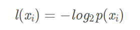
其中,p(xi)是选择该分类的概率
为了计算熵,我们需要计算所有类别所有可能值所包含的信息期望值,通过下式得到:
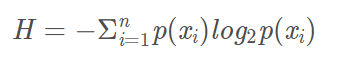
其中,n为分类数目,熵越大,随机变量的不确定性就越大。
from math import log

def calcShannonEnt(dataSet):
    numEntries = len(dataSet)
    print("样本总数:" + str(numEntries))

    labelCounts = {}  # 记录每一类标签的数量

    # 定义特征向量featVec
    for featVec in dataSet:

        currentLabel = featVec[-1]  # 最后一列是类别标签

        if currentLabel not in labelCounts.keys():
            labelCounts[currentLabel] = 0;

        labelCounts[currentLabel] += 1  # 标签currentLabel出现的次数
        print("当前labelCounts状态:" + str(labelCounts))

    shannonEnt = 0.0

    for key in labelCounts:
        prob = float(labelCounts[key]) / numEntries  # 每一个类别标签出现的概率

        print(str(key) + "类别的概率:" + str(prob))
        print(prob * log(prob, 2))
        shannonEnt -= prob * log(prob, 2)
        print("熵值:" + str(shannonEnt))

    return shannonEnt


def createDataSet():
    dataSet = [
        [1, 1, 'yes'],
        [1, 0, 'yes'],
        [1, 1, 'no'],
        [0, 1, 'no'],
        [0, 1, 'no']]

    labels = ['no surfacing', 'flippers']

    return dataSet, labels

def testCalcShannonEnt():
    myDat, labels = createDataSet()
    print(calcShannonEnt(myDat))

if __name__ == '__main__':
    testCalcShannonEnt()
    print(log(0.000002, 2))

得到熵之后,我们就可以按照获取最大信息增益的方法划分数据集
划分数据集
分类算法除了需要测量信息熵,还需要划分数据集,度量划分数据集的熵,以便判断当前是否正确的划分了数据集
# 代码功能:划分数据集
def splitDataSet(dataSet,axis,value): #传入三个参数:待划分的数据集,划分数据集的特征,需要返回的特征的值
    retDataSet = [] #由于参数的链表dataSet我们拿到的是它的地址,也就是引用,直接在链表上操作会改变它的数值,所以我们新建一格链表来做操作

    for featVec in dataSet:
        if featVec[axis] == value: #如果某个特征和我们指定的特征值相等
        #除去这个特征然后创建一个子特征
            reduceFeatVec = featVec[:axis]
            reduceFeatVec.extend(featVec[axis+1:])
            #将满足条件的样本并且经过切割后的样本都加入到我们新建立的样本中
            retDataSet.append(reduceFeatVec)

    return retDataSet
选择最好的数据集划分方式
def chooseBestFeatureToSplit(dataSet):
	# 获取我们样本集中的某一个样本的特征数(因为每一个样本的特征数是相同的,相当于这个代码就是我们可以作为分类依据的所有特征个数)我们的样本最后一列是样本所属的类别,所以要减去类别信息,在我们的例子中特征数就是2
    numFeatures = len(dataSet[0])-1
    #计算样本的初始香农熵
    baseEntropy = calcShannonEnt(dataSet)
    #初始化最大信息增益
    bestInfoGain =0.0
    #最佳划分特征
    bestFeature = -1

    for i in range(numFeatures):
        featList = [sample[i] for sample in dataSet] # 我们首先遍历整个数据集,首先得到第一个特征值可能的取值,然后把它赋值给一个链表,我们第一个特征值取值是[1,1,1,0,0],其实只有【1,0】两个取值
        uniqueVals = set(featList)
        newEntropy = 0.0
        for value in uniqueVals: #uniqueVals中保存的是我们某个样本的特征值的所有的取值的可能性
            subDataSet = splitDataSet(dataSet,i,value)
            prob = len(subDataSet)/float(len(dataSet))
            newEntropy += prob * calcShannonEnt(subDataSet)

        infoGain = baseEntropy - newEntropy# 计算出信息增益

        if(infoGain > bestInfoGain):
            bestInfoGain = infoGain
            bestFeature = i

    return bestFeature
该函数实现选取特征,划分数据集,计算得出最好的划分数据集的特征
信息增益率
信息增益原则对于每个分支节点,都会乘以其权重,也就是说,由于权重之和为1,所以分支节点分的越多,即每个节点数据越小,纯度可能越高。这样会导致信息熵准则偏爱那些取值数目较多的属性。

信息增益率原则可能对取值数目较少的属性更加偏爱,为了解决这个问题,可以先找出信息增益在平均值以上的属性,在从中选择信息增益率最高的。
信息增益比率实际在信息增益的基础上,又将其除以一个值,这个值一般被成为分裂信息量,是将属性可选值m作为划分,计算节点上样本总的信息熵。
基尼系数
基尼系数:表示在样本集合中一个随机选中的样本被分错的概率
基尼系数 = 样本被选中的概率 * 样本被分错的概率
基尼系数的性质与信息熵一样:度量随机变量的不确定度的大小;
G 越大,数据的不确定性越高;
G 越小,数据的不确定性越低;
G = 0,数据集中的所有样本都是同一类别;
分类问题中,假设D有K个类,样本点属于第k类的概率为pk, 则概率 分布的基尼值定义为:

给定数据集D,属性a的基尼指数定义为:

    # 计算某一维度相对于标签的基尼指数
    def Gini(self, y):
        size = len(y) # 数据集大小
        gini_total = 0
        classes_idx_num = dict(Counter(y)) # 统计每类标签下包含的数据个数
        # 计算基尼系数:
        for key in classes_idx_num.keys():
            # 计算第key个标签的基尼系数分量
            prob = classes_idx_num[key] / size # 用出现频率表示概率
            gini_total += prob * prob
        return 1 - gini_total

    def GiniIdx(self, X, y, num_D, dim):
        a = X[:, dim] # 获取数据第dim维度
        v = set(a)    # 获取数据第dim维度可能的取值
        gini_a = 0
        # 计算数据第dim维度的信息增益:
        for i in v:
            # 第dim维度第i个取值出现的频率
            prob_a_v = np.sum(a==i)/num_D
            gini_a_v = self.Gini(y[np.where(a==i)])
            gini_a += prob_a_v * gini_a_v
        return gini_a
X: 输入数据, size=(batches, features)
y: 类别标签, size=(batches,)
dim: 当前是第几维度
num_D: 数据总数
信息熵和基尼系数的比较
- 信息熵的计算比基尼系数的稍慢一些,因为信息熵的公式里是要求log的,而基尼系数公式中只是平方求和而已。
- Scikit Learn中的决策树默认使用基尼系数方式,所以当我们不传入criterion参数时,默认使用gini方式。
- 信息熵和基尼系数没有特别的效果优劣。只是大家需要了解决策树根节点划分的方式原理。
在Python中使用Matplotlib注解绘制树形图
Matplotlib注解
Matplotlib提供了一个注解工具:annotations,可以在数据图形上添加文本工具。
Matplotlib实际上是一套面向对象的绘图库,它所绘制的图表中的每个绘图元素,例如线条Line2D、文字Text、刻度等在内存中都有一个对象与之对应。
import matplotlib.pyplot as plt

decisionNode = dict(boxstyle="sawtooth", fc="0.8") # 决策节点的属性。boxstyle为文本框的类型,sawtooth是锯齿形,fc是边框线粗细
# 可以写为decisionNode={boxstyle:'sawtooth',fc:'0.8'}
leafNode = dict(boxstyle="round4", fc="0.8") #决策树叶子节点的属性
arrow_args = dict(arrowstyle = "<-") #箭头的属性

def plotNode(nodeTxt, centerPt, parentPt, nodeType):
    createPlot.ax1.annotate(nodeTxt, xy=parentPt, xycoords='axes fraction', xytext=centerPt, textcoords='axes fraction',
                            va="center", ha="center", bbox=nodeType, arrowprops=arrow_args)
    #nodeTxt为要显示的文本,centerPt为文本的中心点,parentPt为箭头指向文本的点,xy是箭头尖的坐标,xytest设置注释内容显示的中心位置
    #xycoords和textcoords是坐标xy与xytext的说明(按轴坐标),若textcoords=None,则默认textcoords与xycoords相同,若都未设置,默认为data
    #va/ha设置节点框中文字的位置,va为纵向取值为(u'top', u'bottom', u'center', u'baseline'),ha为横向取值为(u'center', u'right', u'left')

def createPlot():
    fig = plt.figure(1, facecolor = 'white') #创建一个画布,背景为白色
    fig.clf() #画布清空
    #ax1是函数createPlot的一个属性,这个可以在函数里面定义也可以在函数定义后加入也可以
    createPlot.ax1 = plt.subplot(111, frameon = True) #frameon表示是否绘制坐标轴矩形
    plotNode('jue ce', (0.5, 0.1), (0.1, 0.5), decisionNode)
    plotNode('leaf', (0.8, 0.1), (0.3, 0.8), leafNode)
    plt.show()

createPlot()

构造注解树
绘制一颗完整的树需要技巧,虽然我们有坐标,但是如何放置所有的树节点却是个问题。所以我们需要知道有多少个叶节点来确定x轴长度;还需要知道有多少层来确定y轴的高度。
def getNumleafs(mytree): # 获得叶节点数目,输入为我们前面得到的树(字典)
    Numleafs = 0 # 初始化
    firstStr = list(mytree.keys())[0] # 注(a) 获得第一个key值(根节点) 'no surfacing'
    secondDict = mytree[firstStr]  # 获得value值 {0: 'no', 1: {'flippers': {0: 'no', 1: 'yes'}}}
    for key in secondDict.keys(): #  键值:0 和 1
        if type(secondDict[key]).__name__=='dict': # 判断如果里面的一个value是否还是dict
            Numleafs += getNumleafs(secondDict[key]) # 递归调用
        else:
            Numleafs += 1
    return Numleafs

def getTreeDepth(mytree):
    maxDepth = 0
    thisDepth = 0
    firstStr = list(mytree.keys())[0]
    secondDict = mytree[firstStr]
    for key in secondDict.keys(): #  键值:0 和 1
        if type(secondDict[key]).__name__=='dict': # 判断如果里面的一个value是否还是dict
            thisDepth += getTreeDepth(secondDict[key]) # 递归调用
        else:
            Numleafs = 1
        if thisDepth > maxDepth:
            maxDepth = thisDepth
    return maxDepth
可以使用函数retrieveTree输出预先存储的树信息,避免了每次测试代码时都要从数据中创建树的麻烦。
def retrieveTree(i):
    # 用于测试的预定义的树结构
    listOfTrees = [{'no surfacing': {0: 'no', 1: {'flippers': {0: 'no', 1: 'yes'}}}},
                   {'no surfacing': {0: 'no', 1: {'flippers': {0: {'head': {0: 'no', 1: 'yes'}}, 1: 'no'}}}}
                  ]
    return listOfTrees[i]
函数retrieveTree()主要用于测试,返回预定义的树结构
def plotMidText(cntrPt, parentPt, txtString):   #  在两个节点之间的线上写上字
    xMid = (parentPt[0]-cntrPt[0])/2.0 + cntrPt[0]
    yMid = (parentPt[1]-cntrPt[1])/2.0 + cntrPt[1]
    creatPlot.ax1.text(xMid, yMid, txtString)  # text() 的使用

def plotTree(myTree, parentPt, nodeName):  # 画树
    numleafs = getNumleafs(myTree)
    depth = getTreeDepth(myTree)
    firstStr = list(myTree.keys())[0]
    cntrPt = (plotTree.xOff+(0.5/plotTree.totalw+float(numleafs)/2.0/plotTree.totalw), plotTree.yOff)
    plotMidText(cntrPt, parentPt, nodeName)
    plotNode(firstStr, cntrPt, parentPt, decisionNode)
    secondDict = myTree[firstStr]
    plotTree.yOff = plotTree.yOff - 1.0/plotTree.totalD # 减少y的值,将树的总深度平分,每次减少移动一点(向下,因为树是自顶向下画的)
    for key in secondDict.keys():
        if type(secondDict[key]).__name__=='dict':
            plotTree(secondDict[key], cntrPt, str(key))
        else:
            plotTree.xOff = plotTree.xOff + 1.0/plotTree.totalw
            plotNode(secondDict[key], (plotTree.xOff, plotTree.yOff), cntrPt, leafNode)
            plotMidText((plotTree.xOff, plotTree.yOff), cntrPt, str(key))
    plotTree.yOff = plotTree.yOff + 1.0/plotTree.totalD


def creatPlot(inTree):  # 使用的主函数
    fig = plt.figure(1, facecolor='white')
    fig.clf()  # 清空绘图区
    axprops = dict(xticks=[], yticks=[]) # 创建字典 存储=====有疑问???=====
    creatPlot.ax1 = plt.subplot(111, frameon=False, **axprops)
    # 调用poltTree(),plotTree()又依次调用了前面介绍的函数和plotMidText()
    plotTree.totalw = float(getNumleafs(inTree))
    plotTree.totalD = float(getTreeDepth(inTree))  # 创建两个全局变量存储树的宽度和深度
    plotTree.xOff = -0.5/plotTree.totalw # 追踪已经绘制的节点位置 初始值为 将总宽度平分 在取第一个的一半
    plotTree.yOff = 1.0
    plotTree(inTree, (0.5,1.0), '')  # 调用函数,并指出根节点源坐标
    plt.show()

决策树预测隐形眼镜类型
通过网上搜索找到隐形眼镜类型的数据集,它包含了很多患者眼部状况的观察条件以及医生推荐的隐形眼镜类型。隐形眼镜类型包括硬材质(hard)、软材质(soft)以及不适合佩戴隐形眼镜(no lenses)
特征有四个:age(年龄)、prescript(症状)、astigmatic(是否散光)、tearRate(眼泪数量)

这里做一个代码的集合,也是对之前步骤的总结和汇总分析
from math import log
import operator
import matplotlib.pyplot as plt

# 程序清单3-1:计算给定数据集的香农熵(经验熵)
def calcShannonEnt(dataSet):
    numEntries = len(dataSet)
    labelCounts = {}
    for featVec in dataSet:
        currentLabel = featVec[-1]
        if currentLabel not in labelCounts.keys():
            labelCounts[currentLabel] = 0
        labelCounts[currentLabel] += 1
    shannonEnt = 0.0
    for key in labelCounts:
        prob = float(labelCounts[key]) / numEntries
        shannonEnt -= prob * log(prob, 2)
    return shannonEnt


# 程序清单3-2:按照给定特征划分数据集
def splitDataSet(dataSet, axis, value):
    retDataSet = []
    for featVec in dataSet:
        if featVec[axis] == value:
            reducedFeatVec = featVec[:axis]
            reducedFeatVec.extend(featVec[axis + 1:])
            retDataSet.append(reducedFeatVec)
    return retDataSet


# 程序清单3-3:选择最好的数据集划分方式
def chooseBestFeatureToSplit(dataSet):
    numFeatures = len(dataSet[0]) - 1
    baseEntropy = calcShannonEnt(dataSet)
    bestInfoGain = 0.0
    bestFeature = -1
    for i in range(numFeatures):
        featList = [example[i] for example in dataSet]
        uniqueVals = set(featList)
        newEntropy = 0.0
        for value in uniqueVals:
            subDataSet = splitDataSet(dataSet, i, value)
            prob = len(subDataSet) / float(len(dataSet))
            newEntropy += prob * calcShannonEnt(subDataSet)
        infoGain = baseEntropy - newEntropy
        if (infoGain > bestInfoGain):
            bestInfoGain = infoGain
            bestFeature = i
    return bestFeature


# 统计classList中出现此处最多的元素(类标签),即选择出现次数最多的结果
def majorityCnt(classList):
    classCount = {}
    for vote in classList:
        if vote not in classCount.keys():
            classCount[vote] = 0
        classCount[vote] += 1
    sortedClassCount = sorted(classCount.iteritems(), key=operator.itemgetter(1), reverse=True)
    return sortedClassCount[0][0]


# 程序清单3-4:创建决策树
def createTree(dataSet, labels):
    classList = [example[-1] for example in dataSet]
    if classList.count(classList[0]) == len(classList):
        return classList[0]
    if len(dataSet[0]) == 1:
        return majorityCnt(classList)
    bestFeat = chooseBestFeatureToSplit(dataSet)
    bestFeatLabel = labels[bestFeat]
    mytree = {bestFeatLabel: {}}
    del (labels[bestFeat])
    featValues = [example[bestFeat] for example in dataSet]
    uniqueVals = set(featValues)
    for value in uniqueVals:
        subLabels = labels[:]
        mytree[bestFeatLabel][value] = createTree(splitDataSet(dataSet, bestFeat, value), subLabels)
    return mytree


# 程序清单3-5:使用文本注解绘制树节点
# decisionNode = dict(boxstyle = "sawtooth", fc = "0.8")
# leafNode = dict(boxstyle = "round4", fc = "0.8")
# arrow_args = dict(arrowstyle = "<-")

# 程序清单3-5:绘制带箭头的注解
def plotNode(nodeTxt, centerPt, parentPt, nodeType):
    arrow_args = dict(arrowstyle="<-")
    createPlot.ax1.annotate(nodeTxt, xy=parentPt, xycoords='axes fraction', xytext=centerPt,
                            textcoords='axes fraction', va="center", ha="center", bbox=nodeType, arrowprops=arrow_args)


# 程序清单3-5:创建绘图区,计算树形图的全局尺寸
def createPlot(inTree):
    fig = plt.figure(1, facecolor='white')
    fig.clf()
    axprops = dict(xticks=[], yticks=[])
    createPlot.ax1 = plt.subplot(111, frameon=False, **axprops)
    plotTree.totalW = float(getNumLeafs(inTree))
    plotTree.totalD = float(getTreeDepth(inTree))
    plotTree.xOff = -0.5 / plotTree.totalW;
    plotTree.yOff = 1.0
    plotTree(inTree, (0.5, 1.0), '')
    plt.show()


# 程序清单3-6:获取叶节点的数目
def getNumLeafs(myTree):
    numLeafs = 0  # 初始化叶子
    firstStr = list(myTree.keys())[0]
    secondDict = myTree[firstStr]
    for key in secondDict.keys():
        if type(secondDict[key]).__name__ == 'dict':
            numLeafs += getNumLeafs(secondDict[key])
        else:
            numLeafs += 1
    return numLeafs


# 程序清单3-6:获取树的层数
def getTreeDepth(myTree):
    maxDepth = 0
    firstStr = list(myTree.keys())[0]
    secondDict = myTree[firstStr]
    for key in secondDict.keys():
        if type(secondDict[key]).__name__ == 'dict':
            thisDepth = 1 + getTreeDepth(secondDict[key])
        else:
            thisDepth = 1
        if thisDepth > maxDepth:
            maxDepth = thisDepth
    return maxDepth


# 程序清单3-7:标注有向边属性
def plotMidText(cntrPt, parentPt, txtString):
    xMid = (parentPt[0] - cntrPt[0]) / 2.0 + cntrPt[0]
    yMid = (parentPt[1] - cntrPt[1]) / 2.0 + cntrPt[1]
    createPlot.ax1.text(xMid, yMid, txtString, va="center", ha="center", rotation=30)


# 程序清单3-7:绘制决策函数
def plotTree(myTree, parentPt, nodeTxt):
    decisionNode = dict(boxstyle="sawtooth", fc="0.8")
    leafNode = dict(boxstyle="round4", fc="0.8")
    numLeafs = getNumLeafs(myTree)
    defth = getTreeDepth(myTree)
    firstStr = list(myTree.keys())[0]
    cntrPt = (plotTree.xOff + (1.0 + float(numLeafs)) / 2.0 / plotTree.totalW, plotTree.yOff)
    plotMidText(cntrPt, parentPt, nodeTxt)
    plotNode(firstStr, cntrPt, parentPt, decisionNode)
    secondeDict = myTree[firstStr]
    plotTree.yOff = plotTree.yOff - 1.0 / plotTree.totalD
    for key in secondeDict.keys():
        if type(secondeDict[key]) is dict:
            plotTree(secondeDict[key], cntrPt, str(key))
        else:
            plotTree.xOff = plotTree.xOff + 1.0 / plotTree.totalW
            plotNode(secondeDict[key], (plotTree.xOff, plotTree.yOff), cntrPt, leafNode)
            plotMidText((plotTree.xOff, plotTree.yOff), cntrPt, str(key))
    plotTree.yOff = plotTree.yOff + 1.0 / plotTree.totalD


if __name__ == '__main__':
    fr = open('lenses.txt')
    lenses = [inst.strip().split('\t') for inst in fr.readlines()]
    print(lenses)
    lensesLabels = ['age', 'prescript', 'astigmatic', 'tearRate']
    myTree_lenses = createTree(lenses, lensesLabels)
    createPlot(myTree_lenses)
绘制出的树如下图所示:

总结
- 决策树分类器开始处理数据集时,我们首先需要测量集合中数据的不一致性,也就是熵,然后寻找最优方案划分数据集,直到数据集中的所有数据属于同一分类。
- 使用Matplotlib的注解功能,我们可以将存储的树结构转化为易于理解的图形。
- 我们可以通过裁剪决策树,合并相邻的无法产生大量信息增益的叶节点,消除过度匹配问题。
- 决策树算法主要包括三个部分:特征选择、树的生成、树的剪枝。
- 特征选择。特征选择的目的是选取能够对训练集分类的特征。特征选择的关键是准则:信息增益、信息增益比、基尼系数
- 决策树的生成。通常是利用信息增益最大、信息增益比最大、基尼系数最小作为特征选择的准则。从根节点开始,递归的生成决策树。相当于是不断选取局部最优特征,或将训练集分割为基本能够正确分类的子集
- 决策树的剪枝。决策树的剪枝是为了防止树的过拟合,增强其泛化能力。包括预剪枝和后剪枝


 848
848


 被折叠的 条评论
为什么被折叠?
被折叠的 条评论
为什么被折叠?
 到【灌水乐园】发言


