tensorflow2.3实现目标定位(一）

tensorflow2.3实现目标定位

常见图像处理的任务

• 1、分类
  给定一副图像，我们用计算机模型预测图片中有什么对象。
• 2、分类与定位
  我们不仅要知道图片中的对象是什么，还要在对象的附近画一个边框，确定该对象所处的位置。
• 3、语义分割区分到图中每一点像素点，而不仅仅是矩形框框住。
• 4、目标检测
  目标检测简单来说就是回答图片里面有什么？分别在哪里？（并把它们使用矩形框框住）
• 5、实例分割
  实例分割是目标检测和语义分割的结合。相对目标检测的边界框，实例分割可精确到物体的边缘；相对语义分割， 实例分割需要标出图上同一物体的不同个体。

图像定位：
对于单纯的分类问题，比较容易理解，给定一幅图片，我们输出一个标签类别。而定位有点复杂，需要输出四个数字(x,y,w,h)，图像中某一个点的坐标(x,y),以及图像的宽度和高度，有了这四个数字，我们就很容易的找到物体的边框。

The OXford-IIIT Pet Dateset是一个宠物图像数据集，包含37种宠物，每种宠物200张左右图片，包含宠物分类，头部轮廓标注和语义分割。

代码实现

导入包

import tensorflow as tf
import matplotlib.pyplot as plt
from lxml import etree
import glob
import numpy as np
from matplotlib.patches import Rectangle

读取一张图像，打印图像的shape

img = tf.io.read_file('./dataset/images/Abyssinian_1.jpg')
img = tf.image.decode_jpeg(img)
print(img.shape）

• TensorShape([400, 600, 3]

显示图像

plt.imshow(img.numpy())
plt.show()

解码标签，读取标签数据

xml = open('./dataset/annotations/xmls/Abyssinian_1.xml').read()
sel = etree.HTML(xml)

从标签中读取图像的宽度

width = sel.xpath('//size/width/text()')[0]
width

• ‘600’

从标签中读取图像的高度

height = sel.xpath('//size/height/text()')[0]
height

• ‘400’

从标签中读取图像的框的左上角点的x坐标

xmin = sel.xpath('//bndbox/xmin/text()')[0]
xmin

• ‘333’

从标签中读取图像的框的左上角点的y坐标

ymin = sel.xpath('//bndbox/ymin/text()')[0]
ymin

• ‘72’

从标签中读取图像的框的右下角点的x坐标

xmax = sel.xpath('//bndbox/xmax/text()')[0]
xmax

• ‘425’

从标签中读取图像的框的右下角点的y坐标

ymax = sel.xpath('//bndbox/ymax/text()')[0]
ymax

• ‘158’
  从标签中读取的数据的形式都是str型，转换成int型

xmin = int(xmin)
ymin = int(ymin)
xmax = int(xmax)
ymax = int(ymax)
width = int(width)
height = int(height)

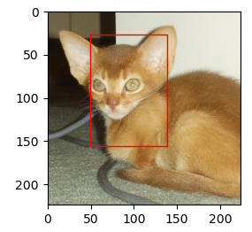
显示图像与定位

plt.imshow(img.numpy())
rect = Rectangle((xmin, ymin), (xmax - xmin), (ymax - ymin), fill=False, color='red')
ax = plt.gca()
ax.axes.add_patch(rect)
plt.show()

测试读取数据，解码， 形状变化，归一化

img = tf.io.read_file('./dataset/images/Abyssinian_1.jpg')
img = tf.image.decode_jpeg(img)
img = tf.image.resize(img, [224, 224])
img = img/255
print(img.shape)

• (224, 224, 3)

读取标注数据，并解码，原图片大小是600400，按比例映射到224224上。

xml = open('./dataset/annotations/xmls/Abyssinian_1.xml').read()
sel = etree.HTML(xml)
width = int(sel.xpath('.//size/width/text()')[0])
height = int(sel.xpath('.//size/height/text()')[0])
xmin = int(sel.xpath('.//bndbox/xmin/text()')[0])
xmax = int(sel.xpath('.//bndbox/xmax/text()')[0])
ymin = int(sel.xpath('.//bndbox/ymin/text()')[0])
ymax = int(sel.xpath('.//bndbox/ymax/text()')[0])
xmin = (xmin/width)*224
xmax = (xmax/width)*224
ymin = (ymin/height)*224
ymax = (ymax/height)*224
print(width, height, xmin, xmax, ymin, ymax)

• 600 400 124.320 158.666 40.32 88.48

把上面读取的图片显示并框出来。

plt.imshow(img)
rect = Rectangle((xmin, ymin), (xmax-xmin), (ymax-ymin), fill=False, color='red')
ax = plt.gca()
ax.axes.add_patch(rect)
plt.show()

创建输入管道

images = glob.glob('./dataset/images/*.jpg')
print(images[:2])
print(len(images))

xmls = glob.glob('./dataset/annotations/xmls/*.xml')
print(xmls[:2])
print(len(xmls))

• [’./dataset/images/samoyed_44.jpg’, ‘./dataset/images/samoyed_102.jpg’]
• 7390
• [’./dataset/annotations/xmls/Maine_Coon_140.xml’, ‘./dataset/annotations/xmls/Egyptian_Mau_104.xml’]
• 3686
  图片数据有7390张，标注的数据只有3686张，所以并不是所有的数据都标注了。下面对数据进行分割，把有标注的图像构造成训练集，没有标注的图像集作为测试集。

训练集

names = [x.split('/')[-1].split('.xml')[0] for x in xmls]
images_train = [img for img in images if (img.split('/')[-1].split('.jpg')[0]) in names]
print(images_train[:2])
print(len(images_train))

• [’./dataset/images/samoyed_102.jpg’,
  ‘./dataset/images/american_pit_bull_terrier_177.jpg’]
• 3686

测试集

images_test = [img for img in images if (img.split('/')[-1].split('.jpg')[0]) not in names]
print(len(images_test))

-3704
3686 + 3704 =7390正好和图像数据大小一致。
为了把图像数据和标签数据是一一对应的，所以按照名称进行排序。

images_train.sort(key=lambda x: x.split('/')[-1].split('.jpg')[0])
print(images_train[:5])
xmls.sort(key=lambda x: x.split('/')[-1].split('.xml')[0])
print(xmls[:5])

• [’./dataset/images/Abyssinian_1.jpg’,
  ‘./dataset/images/Abyssinian_10.jpg’,
  ‘./dataset/images/Abyssinian_100.jpg’,
  ‘./dataset/images/Abyssinian_101.jpg’,
  ‘./dataset/images/Abyssinian_102.jpg’]
• [’./dataset/annotations/xmls/Abyssinian_1.xml’,
  ‘./dataset/annotations/xmls/Abyssinian_10.xml’,
  ‘./dataset/annotations/xmls/Abyssinian_100.xml’,
  ‘./dataset/annotations/xmls/Abyssinian_101.xml’,
  ‘./dataset/annotations/xmls/Abyssinian_102.xml’]

结果显示是一一对应的。

上面是label测试方法的可行性，下面自定义一个封装函数，把以上过程封装在一起。

def to_labels(path):
    xml = open('{}'.format(path)).read()
    sel = etree.HTML(xml)
    width = int(sel.xpath('.//size/width/text()')[0])
    height = int(sel.xpath('.//size/height/text()')[0])
    xmin = int(sel.xpath('.//bndbox/xmin/text()')[0])
    xmax = int(sel.xpath('.//bndbox/xmax/text()')[0])
    ymin = int(sel.xpath('.//bndbox/ymin/text()')[0])
    ymax = int(sel.xpath('.//bndbox/ymax/text()')[0])
    return [xmin / width, ymin / height, xmax / width, ymax / height]

把标注数据应用到这个封装函数上

labels = [to_labels(path) for path in xmls]
print(labels[:3]）

• [[0.555, 0.18, 0.708, 0.395],
  [0.192, 0.21, 0.768, 0.582],
  [0.3832, 0.142, 0.850, 0.534]]
  目前的label中把四个数值放在一个序列里，我们输入时要把四个值每一个值作为一个列表所以要反序列压缩

out1, out2, out3, out4 = list(zip(*labels))
out1 = np.array(out1)
out2 = np.array(out2)
out3 = np.array(out3)
out4 = np.array(out4)

构建label集

label_dataset = tf.data.Dataset.from_tensor_slices((out1, out2, out3, out4))

封装读取图像数据函数

def load_image(path):
    img = tf.io.read_file(path)
    img = tf.image.decode_jpeg(img, channels=3)
    img = tf.image.resize(img, [224, 224])
    img = img/127.5 - 1           #-1～1
    return img

构造图像数据训练集，并应用到读取函数上

image_dataset = tf.data.Dataset.from_tensor_slices(images_train)
image_dataset = image_dataset.map(load_image)

把图像数据和目标标注数据zip到一个dataset中

dataset = tf.data.Dataset.zip((image_dataset, label_dataset))

数据进行训练时要重复和循环

dataset = dataset.repeat().shuffle(len(images_train)).batch(32)

设置训练集中训练和测试的数量

test_count = int(len(images_train) * 0.2)
train_count = len(images_train) - test_count
train_dataset = dataset.skip(test_count)
test_dataset = dataset.take(test_count)

创建模型
利用Xception预训练模型，添加全连接曾，全连接曾不能是四维，所以在之前要进行GlobalAveragePooling2D

xception = tf.keras.applications.xception.Xception(weights='imagenet', include_top=False, input_shape=(224, 224, 3))
inputs = tf.keras.layers.Input(shape=(224, 224, 3))
x = xception(inputs)
x = tf.keras.layers.GlobalAveragePooling2D()(x)
x = tf.keras.layers.Dense(2048, activation='relu')(x)
x = tf.keras.layers.Dense(256, activation='relu')(x)
out1 = tf.keras.layers.Dense(1)(x)
out2 = tf.keras.layers.Dense(1)(x)
out3 = tf.keras.layers.Dense(1)(x)
out4 = tf.keras.layers.Dense(1)(x)

没有经过训练可以进行预测

prediction = [out1, out2, out3, out4]

模型配置和训练

model = tf.keras.models.Model(inputs=inputs, outputs=prediction)
model.compile(optimizer=tf.keras.optimizers.Adam(lr=0.0001), loss='mse', metrics=['mae'])
history = model.fit(train_dataset, epochs=5, steps_per_epoch=train_count//64, validation_data=test_dataset, validation_steps=test_count//64)

模型保存，可以把训练好的模型保存下来

 model.save('detect_v1.h5')

下次使用时，加载已经训练好的模型

new_model = 
tf.keras.models.load_model('detect_v1.h5')

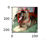
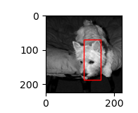
预测

plt.figure(figsize=(20, 8))
for img, _ in test_dataset.take(1):
    out1, out2, out3, out4 = model.predict(img)
    for i in range(3):
        plt.subplot(3, 1, i+1)
        plt.imshow(tf.keras.preprocessing.image.array_to_img(img[i]))
        xmin, ymin, xmax, ymax =out1[i]*224, out2[i]*224, out3[i]*224, out4[i]*224
        rect = Rectangle((xmin, ymin), (xmax - xmin), (ymax - ymin), fill=False, color='red')
        ax = plt.gca()
        ax.axes.add_patch(rect)
        plt.show()