机器学习实践—基于Scikit-Learn、Keras和TensorFlow2第二版—第6章 决策树(Decision Trees)

与SVM类似，决策树可以完成分类和回归任务，甚至可以完成多输出任务。

决策树也是随机森林的基础组成部分，随机森林就是通过组合不同的大小(深度)的决策树达到很好的效果。

0. 导入所需的库

import sklearn
import numpy as np
import matplotlib as mpl
%matplotlib inline
import matplotlib.pyplot as plt
import os

for i in (sklearn, np, mpl):
    print(i.__name__,": ",i.__version__,sep="")

输出：

sklearn: 0.21.3
numpy: 1.17.4
matplotlib: 3.1.2

1. 决策树模型的训练与可视化

导入数据集：

from sklearn.datasets import load_iris
from sklearn.tree import DecisionTreeClassifier

iris = load_iris()
X = iris.data[:,2:]
y = iris.target

X.shape, y.shape

输出：

((150, 2), (150,))

tree_clf = DecisionTreeClassifier(max_depth=2, random_state=42)
tree_clf.fit(X,y)

输出：

DecisionTreeClassifier(class_weight=None, criterion='gini', max_depth=2,
                       max_features=None, max_leaf_nodes=None,
                       min_impurity_decrease=0.0, min_impurity_split=None,
                       min_samples_leaf=1, min_samples_split=2,
                       min_weight_fraction_leaf=0.0, presort=False,
                       random_state=42, splitter='best')

from graphviz import Source
from sklearn.tree import export_graphviz

image_path = "./images/decision_trees"
os.makedirs(image_path, exist_ok=True)

export_graphviz(tree_clf,
               out_file=os.path.join(image_path,"iris_tree.dot"),
               feature_names=iris.feature_names[2:],
               class_names=iris.target_names,
               rounded=True,
               filled=True)
Source.from_file(os.path.join(image_path,"iris_tree.dot"))

输出：

如上所示为构建的决策树模型，通过以上构建决策树模型发现，决策树算法不要求训练集归一化和中心化。

2. 决策树模型预测

上述图中，节点的samples属性表示属于训练集中属于该节点的样本个数，value属性表示属于该节点的每个类别的样本个数，gini属性表示样本类别的混杂度，例如所有样本属于一个类别的，则gini等于1，如果属于两个类别并各占一半，则gini等于0.5。gini计算公式如下：

from matplotlib.colors import ListedColormap

def plot_decision_boundary(clf, X, y, axes=[0,7.5, 0, 3], iris=True, legend=False, plot_training=True):
    x1s = np.linspace(axes[0], axes[1],100)
    x2s = np.linspace(axes[2], axes[3],100)
    x1, x2 = np.meshgrid(x1s, x2s)
    
    X_new = np.c_[x1.ravel(), x2.ravel()]
    y_pred = clf.predict(X_new).reshape(x1.shape)
    custom_cmap = ListedColormap(['#fafab0','#9898ff','#a0faa0'])
    plt.contourf(x1, x2, y_pred, alpha=0.3, cmap=custom_cmap)
    
    if not iris:
        custom_cmap2 = ListedColormap(['#7d7d58','#4c4c7f','#507d50'])
        plt.contourf(x1, x2, y_pred, cmap=custom_cmap2, alpha=0.8)
    if plot_training:
        plt.plot(X[:,0][y==0],X[:,1][y==0],"yo",label="Iris setosa")
        plt.plot(X[:,0][y==1],X[:,1][y==1],"bs",label="Iris versicolor")
        plt.plot(X[:,0][y==2],X[:,1][y==2],"g^",label="Iris virginica")
        plt.axis(axes)
    if iris:
        plt.xlabel("Petal Length", fontsize=14)
        plt.ylabel("Petal Width",fontsize=14)
    else:
        plt.xlabel(r"$x_1$",fontsize=18)
        plt.ylabel(r"$x_2$",fontsize=18,rotation=0)
    if legend:
        plt.legend(fontsize=14)
    
plt.figure(figsize=(12,6))
plot_decision_boundary(tree_clf, X, y)

plt.plot([2.45,2.45],[0,3],"k-",linewidth=5)
plt.text(1.70,1.0,"Depth=0",fontsize=15)
plt.plot([2.45,7.5],[1.75,1.75],"k--",linewidth=5)
plt.text(3.8,1.8,"Depth=1",fontsize=15)

plt.plot([4.85,4.85],[1.75,3],"g--",linewidth=3)
plt.plot([4.955,4.955],[0,1.75],"r--",linewidth=3)
plt.text(4.2,0.5,"(Depth=2)",fontsize=15)

plt.tight_layout()
plt.show()

输出：

如上图所示为决策树的决策边界。

黑色直线表示根节点的决策边界，即花瓣长度2.45cm。可以看到，黑色直线左边是一类，右边是两类，所以还需要在右边找到一条直线将蓝色点和绿色点分开。

黑色虚线表示第一层右边节点的决策边界，即花瓣宽度1.75cm。可以看到，决策边界将大部分样本分开了，但有少数蓝色点和绿色点分错了。

如果设置较大的深度，例如模型构建时设置超参数max_depth=3，则可能第二层节点会继续分下去，例如如图中红色虚线和绿色虚线所示，其中绿色虚线为第二层右边节点的决策边界，而红色虚线为第二层左边节点的决策边界。

3. 预测类别及类别概率

决策树模型也可以输出预测样本属于某个类的概率值，这个概率值就是根据节点中value值计算的：

tree_clf.predict_proba([[5,1.5]])

输出：

array([[0.        , 0.90740741, 0.09259259]])

tree_clf.predict([[5,1.5]])

输出：

array([1])

如上输出结果显示，当预测样本花瓣长度为5，宽度为1.5时，则根据上面训练的决策树模型，该样本会落到第二层左边的节点上，则概率分别为0/54=0，49/54=90.7，5/54=9.3%，观察发现与上面的输出一致。

4. CART算法

sklearn使用CART算法进行决策树的训练，CART主要思想就是找到两个子集，使得加权生的纯度最高。找到两个子集后再分别对这两个子集找子集，以次类推，直到达到超参数规定的最大深度，或者无法找到两个加权求和之后的纯度更高的子集。或者可以使用其它超参数控制CART算法的终止，例如min_sampes_split，max_leaf_nodes等。

注意：CART算法属于贪婪算法。贪婪算法通常能生成比较好的解决方案，但不保证是最佳的。找到最佳的决策树属于NP-完问题范畴，计算复杂度为O(exp(m))，这对于很小的数据集都比较棘手，更不用对中大型数据集了。

5. 计算复杂度

用决策树预测较大数据集时，运算速度也比较快。预测样本只需要在每层的两个节点中选一个，并且根据所有特征中的一个特征判断选择下一层的哪个节点，因此预测计算复杂度为O(log2(m))。

训练复杂度为O(nmlog2(m))，在每一层需要比较所有样本的所有特征。

6. gini系数

sklearn中默认使用gini 纯度为判断标准，也可以手动指定gini熵(criterion=entropy)为判断标准。

熵的概念源于热力学，其用来表征分子无序的一种度量，当分子处理静止且有序时，熵为0。后来被广泛应用于其它领域，例如香农信息学领域，用来表征信息的一致程度。

在机器学习中，熵的含义是如果样本都属于一个类别，则熵为0，计算公式如下：

7. 正则化超参数

决策树算法几乎对训练数据没什么要求，决策树会尽可能地去拟合训练数据，因此过拟合是决策树经常发生的问题。

sklearn中可以通过max_depth超参数设置树的最大深度，min_samples_split节点中样本个数大于这个值时才会继续分隔，min_samples_leaf叶子节点最小样本个数，等等。

from sklearn.datasets import make_moons

Xm, ym = make_moons(n_samples=100, noise=0.25, random_state=53)

deep_tree_clf1 = DecisionTreeClassifier(random_state=42)
deep_tree_clf2 = DecisionTreeClassifier(min_samples_leaf=4, random_state=42)
deep_tree_clf1.fit(Xm, ym)
deep_tree_clf2.fit(Xm, ym)

fig, axes = plt.subplots(ncols=2, figsize=(12, 5), sharey=True)

plt.sca(axes[0])
plot_decision_boundary(deep_tree_clf1, Xm, ym, axes=[-1.5, 2.4, -1, 1.5], iris=False)
plt.title("No restrictions", fontsize=16)

plt.sca(axes[1])
plot_decision_boundary(deep_tree_clf2, Xm, ym, axes=[-1.5, 2.4, -1, 1.5], iris=False)
plt.title("min_samples_leaf = {}".format(deep_tree_clf2.min_samples_leaf), fontsize=14)
plt.ylabel("")

plt.tight_layout()
plt.show()

输出：

如上输出，左图模型使用sklearn默认超参数，右图模型为指定叶节节点样本个数大于等于4。观察发现，左图有明显的过拟合，而右图模型是比较好的结果。

angle = np.pi / 180 * 20
rotation_matrix = np.array([[np.cos(angle), -np.sin(angle)], [np.sin(angle), np.cos(angle)]])
Xr = X.dot(rotation_matrix)

tree_clf_r = DecisionTreeClassifier(random_state=42)
tree_clf_r.fit(Xr, y)

plt.figure(figsize=(12, 5))
plot_decision_boundary(tree_clf_r, Xr, y, axes=[0.5, 7.5, -1.0, 1], iris=False)

plt.show()

输出：

8. 决策树完成回归任务

决策树不仅能完成分类任务，也能完成回归任务。

np.random.seed(42)
m=200

X = np.random.rand(m,1)
y = 4 * (X-0.5)**2
y = y + np.random.randn(m,1)/10

X.shape, y.shape

输出：

((200, 1), (200, 1))

from sklearn.tree import DecisionTreeRegressor

tree_reg = DecisionTreeRegressor(max_depth=2, random_state=42)
tree_reg.fit(X,y)

输出：

DecisionTreeRegressor(criterion='mse', max_depth=2, max_features=None,
                      max_leaf_nodes=None, min_impurity_decrease=0.0,
                      min_impurity_split=None, min_samples_leaf=1,
                      min_samples_split=2, min_weight_fraction_leaf=0.0,
                      presort=False, random_state=42, splitter='best')

export_graphviz(tree_reg,
               out_file=os.path.join(image_path,"regression_tree.dot"),
               feature_names=["x1"],
               rounded=True,
               filled=True)
Source.from_file(os.path.join(image_path,"regression_tree.dot"))

输出：

生成的决策树如上图所示。从形状上看起来与决策树分类模型很类似，区别在于决策树分类模型返回的是预测的类别，而决策树回归模型返回的数值。

那么，决策树回归模型是如何预测的呢？假如有预测样本x=0.6，则根据上面决策树会落到第二层第三个节点上，那么预测的结果就是0.111。这个0.111是训练过程中落到这个节点上的110个样本的平均值，并且这110个样本的均方差是0.015。

tree_reg1 = DecisionTreeRegressor(random_state=42, max_depth=2)
tree_reg2 = DecisionTreeRegressor(random_state=42, max_depth=3)
tree_reg1.fit(X,y)
tree_reg2.fit(X,y)

def plot_regression_predictions(tree_reg, X, y, axes=[0,1,-0.2,1], ylabel="$y$"):
    x1 = np.linspace(axes[0], axes[1],500).reshape(-1,1)
    y_pred = tree_reg.predict(x1)
    plt.axis(axes)
    plt.xlabel("$x_1$",fontsize=18)
    if ylabel:
        plt.ylabel(ylabel, fontsize=18, rotation=0)
    plt.plot(X,y,"b.")
    plt.plot(x1, y_pred, "r.-",linewidth=2, label=r"$\hat{y}$")
    
fig, axes = plt.subplots(ncols=2,figsize=(12,5),sharey=True)

plt.sca(axes[0])
plot_regression_predictions(tree_reg1, X, y)
plt.legend(fontsize=18)
for split, style in ((0.1973, "k-"), (0.0917, "k--"), (0.7718, "k--")):
    plt.plot([split, split], [-0.2, 1], style, linewidth=2)
plt.text(0.21, 0.65, "Depth=0", fontsize=15)
plt.text(0.01, 0.2, "Depth=1", fontsize=13)
plt.text(0.65, 0.8, "Depth=1", fontsize=13)
plt.title("max_depth=2", fontsize=14)

plt.sca(axes[1])
plot_regression_predictions(tree_reg2, X, y, ylabel=None)
plt.legend(fontsize=18)
plt.title("max_depth=3",fontsize=14)
for split, style in ((0.1973, "k-"), (0.0917, "k--"), (0.7718, "k--")):
    plt.plot([split, split], [-0.2, 1], style, linewidth=2)
for split in (0.0458, 0.1298, 0.2873, 0.9040):
    plt.plot([split, split], [-0.2, 1], "k:", linewidth=1)
plt.text(0.3, 0.5, "Depth=2", fontsize=13)

plt.tight_layout()
plt.show()

输出：

如上图所示，左图是最大深度为2的决策树回归模型，右图是最大深度为3的决策树回归模型。

CART与之前的类似，目标是不断地拆分训练集，使得圴方误差MSE最小。

与决策树分类算法类似，决策树回归模型也同样很容易过拟合：

tree_reg1 = DecisionTreeRegressor(random_state=42)
tree_reg2 = DecisionTreeRegressor(random_state=42, min_samples_leaf=10)
tree_reg1.fit(X, y)
tree_reg2.fit(X, y)

x1 = np.linspace(0, 1, 500).reshape(-1, 1)
y_pred1 = tree_reg1.predict(x1)
y_pred2 = tree_reg2.predict(x1)

fig, axes = plt.subplots(ncols=2, figsize=(12, 5), sharey=True)

plt.sca(axes[0])
plt.plot(X, y, "b.")
plt.plot(x1, y_pred1, "r.-", linewidth=2, label=r"$\hat{y}$")
plt.axis([0, 1, -0.2, 1.1])
plt.xlabel("$x_1$", fontsize=18)
plt.ylabel("$y$", fontsize=18, rotation=0)
plt.legend(loc="upper center", fontsize=18)
plt.title("No restrictions", fontsize=14)

plt.sca(axes[1])
plt.plot(X, y, "b.")
plt.plot(x1, y_pred2, "r.-", linewidth=2, label=r"$\hat{y}$")
plt.axis([0, 1, -0.2, 1.1])
plt.xlabel("$x_1$", fontsize=18)
plt.title("min_samples_leaf={}".format(tree_reg2.min_samples_leaf), fontsize=14)

plt.tight_layout()
plt.show()

输出：

如上输出所示，左图为使用sklearn默认的参数，右图为指定超参数min_samples_leaf=10。观察可以发现，使用默认参数的左图模型很明显处理过拟合状态，右图模型效果似乎稍微好一些。

9. 不稳定性

决策树易于理解，解释性强，容易使用并且功能比较强大。但是，也有一些缺点或不足：

一是决策树决策边界都是正交的，即决策边界都垂直于坐标轴。换句话说，决策树模型对训练集的方向（或旋转）比较敏感。请看下面这个例子：

np.random.seed(6)

Xs = np.random.rand(100, 2) - 0.5
ys = (Xs[:, 0] > 0).astype(np.float32) * 2

angle = np.pi / 4
rotation_matrix = np.array([[np.cos(angle), -np.sin(angle)], [np.sin(angle), np.cos(angle)]])
Xsr = Xs.dot(rotation_matrix)

tree_clf_s = DecisionTreeClassifier(random_state=42)
tree_clf_s.fit(Xs, ys)
tree_clf_sr = DecisionTreeClassifier(random_state=42)
tree_clf_sr.fit(Xsr, ys)

fig, axes = plt.subplots(ncols=2, figsize=(12, 5), sharey=True)
plt.sca(axes[0])
plot_decision_boundary(tree_clf_s, Xs, ys, axes=[-0.7, 0.7, -0.7, 0.7], iris=False)

plt.sca(axes[1])
plot_decision_boundary(tree_clf_sr, Xsr, ys, axes=[-0.7, 0.7, -0.7, 0.7], iris=False)
plt.ylabel("")

plt.tight_layout()
plt.show()

输出：

如上输出所示，左图为原始数据训练的决策树分类模型，分类效果很好。右图是将训练数据进行了45度的旋转，此时模型就变得很复杂，需要5条决策边界才能将数据分开。对于右图数据，如果使用线性回归模型，一条直接几乎很轻松就能把两个类别分开。

二是决策树模型对训练数据细微的变化很敏感。请看下面这个例子：

X[(X[:, 1]==X[:, 1][y==1].max()) & (y==1)] # 花瓣最宽的Iris versicolor

not_widest_versicolor = (X[:, 1]!=1.8) | (y==2)  # 从数据集中删除花瓣最宽的数据
X_tweaked = X[not_widest_versicolor]
y_tweaked = y[not_widest_versicolor]

tree_clf_tweaked = DecisionTreeClassifier(max_depth=2, random_state=40)
tree_clf_tweaked.fit(X_tweaked, y_tweaked)

输出：

DecisionTreeClassifier(class_weight=None, criterion='gini', max_depth=2,
                       max_features=None, max_leaf_nodes=None,
                       min_impurity_decrease=0.0, min_impurity_split=None,
                       min_samples_leaf=1, min_samples_split=2,
                       min_weight_fraction_leaf=0.0, presort=False,
                       random_state=40, splitter='best')

plt.figure(figsize=(12,5))

plt.subplot(122)
plot_decision_boundary(tree_clf_tweaked, X_tweaked, y_tweaked, legend=False)

plt.plot([0, 7.5], [0.8, 0.8], "k-", linewidth=2)
plt.plot([0, 7.5], [1.75, 1.75], "k--", linewidth=2)
plt.text(1.0, 0.9, "Depth=0", fontsize=15)
plt.text(1.0, 1.80, "Depth=1", fontsize=13)
plt.ylabel("")
plt.title("Non Widest versicolor")

plt.subplot(121)
plot_decision_boundary(tree_clf, X, y, legend=False)
plt.title("All datasets")
plt.plot([2.45, 2.45], [0, 3], "k-", linewidth=2)
plt.plot([2.45, 7.5], [1.75, 1.75], "k--", linewidth=2)
plt.text(1.10, 1.0, "Depth=0", fontsize=15)
plt.text(3.2, 1.80, "Depth=1", fontsize=13)

plt.tight_layout()
plt.show()

输出：

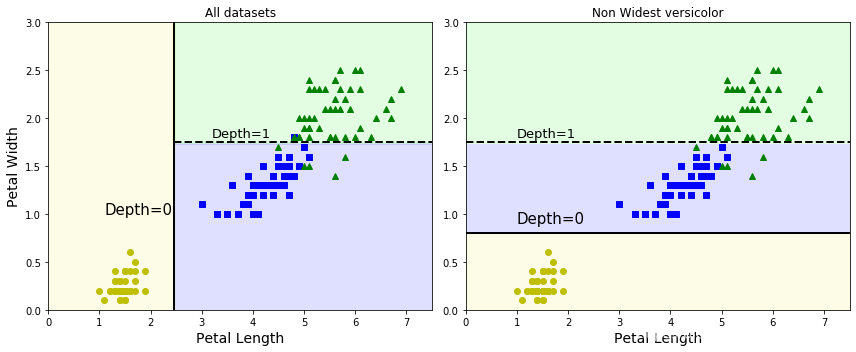
如上输出所示，左图是原始数据上训练的决策树模型，而右图是删除最宽花瓣的数据后训练的决策模型，对比左右模型发现，两者是完全不同的两个模型。说明决策树模型对训练数据微小的变化很敏感。

同时，sklearn中决策树的训练算法是随机的，利用相同的数据训练决策树模型，每次得到的结果可能都不一样。可以通过设置超参数random_state，可保证每次的随机性一样，类似于随机种子的功能。