


https://graphsandnetworks.com/the-cora-dataset/
Graph Convolutional Network (GCN) on the CORA citation dataset — StellarGraph 1.0.0rc1 documentation
pytorch-GAT/The Annotated GAT (Cora).ipynb at main · gordicaleksa/pytorch-GAT · GitHub

Cora数据集
Cora数据集包括2708份科学出版物,分为7类。引文网络由5429个链接组成。数据集中的每个发布都用一个0/1值的词向量来描述,该词向量表示字典中相应词的缺失/存在。这部词典由1433个独特的单词组成。
这个数据集在图学习中是MNIST等价的。
import pandas as pd

node_df = pd.read_csv('./data/nodes.csv')
node_df.head()| Unnamed: 0 | nodeId | labels | subject | features | |
|---|---|---|---|---|---|
| 0 | 0 | 31336 | Paper | Neural_Networks | [0, 0, 0, 0, 0, 0, 0, 0, 0, 0, 0, 0, 0, 0, 0, ... |
| 1 | 1 | 1061127 | Paper | Rule_Learning | [0, 0, 0, 0, 0, 0, 0, 0, 0, 0, 0, 0, 1, 0, 0, ... |
| 2 | 2 | 1106406 | Paper | Reinforcement_Learning | [0, 0, 0, 0, 0, 0, 0, 0, 0, 0, 0, 0, 0, 0, 0, ... |
| 3 | 3 | 13195 | Paper | Reinforcement_Learning | [0, 0, 0, 0, 0, 0, 0, 0, 0, 0, 0, 0, 0, 0, 0, ... |
| 4 | 4 | 37879 | Paper | Probabilistic_Methods | [0, 0, 0, 0, 0, 0, 0, 0, 0, 0, 0, 0, 0, 0, 0, ... |
edge_df = pd.read_csv('./data/edges.csv')
edge_df.head()| Unnamed: 0 | sourceNodeId | targetNodeId | relationshipType | |
|---|---|---|---|---|
| 0 | 0 | 35 | 1033 | CITES |
| 1 | 1 | 35 | 103482 | CITES |
| 2 | 2 | 35 | 103515 | CITES |
| 3 | 3 | 35 | 1050679 | CITES |
| 4 | 4 | 35 | 1103960 | CITES |
edge_df = pd.read_csv('./data/edges.csv', names=["target", "source"])
edge_df["label"] = "cites"

edge_df.sample(frac=0.5).head(5)| target | source | label | ||
|---|---|---|---|---|
| 563.0 | 2354 | 1130539 | CITES | cites |
| 2766.0 | 35061 | 32083 | CITES | cites |
| 4040.0 | 1107808 | 116512 | CITES | cites |
| 134.0 | 594543 | 35 | CITES | cites |
| 1023.0 | 4584 | 124064 | CITES | cites |
https://graphsandnetworks.com/the-cora-dataset/
按此指引,下载

https://github.com/gordicaleksa/pytorch-GAT/blob/main/The%20Annotated%20GAT%20(Cora).ipynb
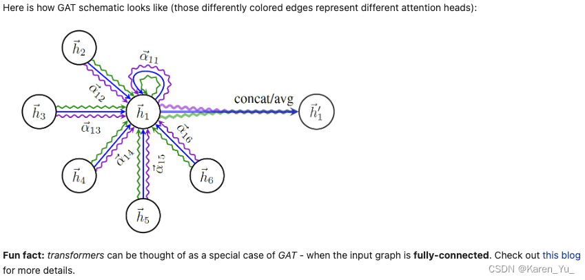
事实证明,将注意力的想法与已经存在的图形卷积网络(GCN)结合起来是一个很好的举动🤓- GAT是GNN文献中被引用次数第二多的论文(截至该notebook撰写时)。
整个想法来自cnn。卷积神经网络解决了各种计算机视觉任务,并在深度学习领域掀起了一场巨大的热潮,所以一些人决定把这个想法转移到图上。基本问题是,虽然图像位于规则网格上(你也可以将其视为图形),因此具有精确的顺序概念,但图不享受这种良好的属性,邻居的数量以及邻居的顺序。
因此,如何定义图的kernel成为一个问题。我们无法建党将kernel的大小定义为,因为节点的邻居可能很少或者很大。
此时主要用到的是两个思路:
- spectral methods(都以某种方式利用了图的拉普拉斯特征基)
据说其历史源于graph signal processing,有空读一下 - spatial method
对于spatial methods(空间方法)的high level解释
假设我们有邻居的特征向量,则可以执行以下操作:
- 以某种方式变换它们(也许是一个线性投影),
- 以某种方式聚合它们(也许用注意力系数对它们进行加权->GAT)。
- 通过将当前节点的(变换后的)特征向量与聚合的邻域表示结合起来,(以某种方式)更新当前节点的特征向量。
import & 读取数据
# I always like to structure my imports into Python's native libs,
# stuff I installed via conda/pip and local file imports (but we don't have those here)

import pickle

# Visualization related imports
import matplotlib.pyplot as plt
import networkx as nx
import igraph as ig

# Main computation libraries
import scipy.sparse as sp
import numpy as np

# Deep learning related imports
import torch
"""
Contains constants needed for data loading and visualization.
"""
import os
import enum
# Supported datasets - only Cora in this notebook
class DatasetType(enum.Enum):
CORA = 0
# Networkx is not precisely made with drawing as its main feature but I experimented with it a bit
class GraphVisualizationTool(enum.Enum):
NETWORKX = 0,
IGRAPH = 1
# We'll be dumping and reading the data from this directory
DATA_DIR_PATH = os.path.join(os.getcwd(), 'data')
CORA_PATH = os.path.join(DATA_DIR_PATH, 'cora') # this is checked-in no need to make a directory
#
# Cora specific constants
#
# Thomas Kipf et al. first used this split in GCN paper and later Petar Veličković et al. in GAT paper
CORA_TRAIN_RANGE = [0, 140] # we're using the first 140 nodes as the training nodes
CORA_VAL_RANGE = [140, 140+500]
CORA_TEST_RANGE = [1708, 1708+1000]
CORA_NUM_INPUT_FEATURES = 1433
CORA_NUM_CLASSES = 7
# Used whenever we need to visualzie points from different classes (t-SNE, CORA visualization)
cora_label_to_color_map = {0: "red", 1: "blue", 2: "green", 3: "orange", 4: "yellow", 5: "pink", 6: "gray"}数据所在位置在当前notebook所在位置data文件夹下后cora文件夹,如:GNN_test_project/data/cora/node_features.csr
使用前140个节点来训练节点,500个节点作为验证,1000个节点作为测试。
输入的feature数量是1433,共分成7类。
为了方便可视化,这里设置了每个类别不同的颜色。
数据集了解
Transductive(直推式) - 假设我们有一个单一的图(如:Cora),将一些节点(而不是图)分成训练/验证/测试训练集。在训练时,只使用来自训练节点的标签。但是。在前向传递过程中,根据空间gnn工作的本质,将从邻居中聚集特征向量,其中一些可能属于验证集甚至测试集!重点是——此处不是在使用它们的标签信息(没有使用节点的feature),而是在使用它们的结构信息和特征。
Inductive(归纳式) - 如果有计算机视觉或NLP背景,可能对这个更熟悉。有一组训练图,有一组单独的验证图当然还有一组单独的测试图。
pickle.load(file)pickle — Python object serialization — Python 3.12.3 documentation
pickle.dump和pickle.load-CSDN博客
从file中读取一个字符串,并重构为原来的python对象
with open(path, 'rb') as filehttps://www.quora.com/What-does-opening-a-file-rb-in-Python-mean
請問with open() as f 的語法意思為何? open()內參數何時使用'wb'、'rb'? - Cupoy
r将字符串字面值标记为raw(在这种特殊情况下不做任何事情),而b将其标记为二进制,这意味着结果对象是bytes对象,而不是STR对象
简单来说就是:读入,并且转换成bytes类型
with open(path, 'wb') as file类似的,这里是写入
pickle.dump(data, file, protocol=pickle.HIGHEST_PROTOCOL)用于将python独享序列化并保存到文件中
loading/saving Pickle files:
# First let's define these simple functions for loading/saving Pickle files - we need them for Cora

# All Cora data is stored as pickle
def pickle_read(path):
    with open(path, 'rb') as file:
        data = pickle.load(file)

    return data

def pickle_save(path, data):
    with open(path, 'wb') as file:
        pickle.dump(data, file, protocol=pickle.HIGHEST_PROTOCOL)
加载数据
node_features_csr = pickle_read(os.path.join(CORA_PATH, 'node_features.csr'))
node_labels_npy = pickle_read(os.path.join(CORA_PATH, 'node_labels.npy'))
adjacency_list_dict = pickle_read(os.path.join(CORA_PATH, 'adjacency_list.dict'))
获得三个数据:
1. 节点特征
2. 边的标签
3. 邻接表(N个节点:节点的所有邻居节点)
load_graph_data
# We'll pass the training config dictionary a bit later
def load_graph_data(training_config, device):
    dataset_name = training_config['dataset_name'].lower()
    should_visualize = training_config['should_visualize']

    if dataset_name == DatasetType.CORA.name.lower():

        # shape = (N, FIN), where N is the number of nodes and FIN is the number of input features
        node_features_csr = pickle_read(os.path.join(CORA_PATH, 'node_features.csr'))
        # shape = (N, 1)
        node_labels_npy = pickle_read(os.path.join(CORA_PATH, 'node_labels.npy'))
        # shape = (N, number of neighboring nodes) <- this is a dictionary not a matrix!
        adjacency_list_dict = pickle_read(os.path.join(CORA_PATH, 'adjacency_list.dict'))

        # Normalize the features (helps with training)
        node_features_csr = normalize_features_sparse(node_features_csr)
        num_of_nodes = len(node_labels_npy)

        # shape = (2, E), where E is the number of edges, and 2 for source and target nodes. Basically edge index
        # contains tuples of the format S->T, e.g. 0->3 means that node with id 0 points to a node with id 3.
        topology = build_edge_index(adjacency_list_dict, num_of_nodes, add_self_edges=True)

        # Note: topology is just a fancy way of naming the graph structure data
        # (aside from edge index it could be in the form of an adjacency matrix)

        if should_visualize:  # network analysis and graph drawing
            plot_in_out_degree_distributions(topology, num_of_nodes, dataset_name)  # we'll define these in a second
            visualize_graph(topology, node_labels_npy, dataset_name)

        # Convert to dense PyTorch tensors

        # Needs to be long int type because later functions like PyTorch's index_select expect it
        topology = torch.tensor(topology, dtype=torch.long, device=device)
        node_labels = torch.tensor(node_labels_npy, dtype=torch.long, device=device)  # Cross entropy expects a long int
        node_features = torch.tensor(node_features_csr.todense(), device=device)

        # Indices that help us extract nodes that belong to the train/val and test splits
        train_indices = torch.arange(CORA_TRAIN_RANGE[0], CORA_TRAIN_RANGE[1], dtype=torch.long, device=device)
        val_indices = torch.arange(CORA_VAL_RANGE[0], CORA_VAL_RANGE[1], dtype=torch.long, device=device)
        test_indices = torch.arange(CORA_TEST_RANGE[0], CORA_TEST_RANGE[1], dtype=torch.long, device=device)

        return node_features, node_labels, topology, train_indices, val_indices, test_indices
    else:
        raise Exception(f'{dataset_name} not yet supported.')
读取节点特征数据,节点特征归一化
读取邻接列表,得到边的连接信息
两者数据类型都是numpy.ndarray
normalize features sparse
def normalize_features_sparse(node_features_sparse):
    assert sp.issparse(node_features_sparse), f'Expected a sparse matrix, got {node_features_sparse}.'

    # Instead of dividing (like in normalize_features_dense()) we do multiplication with inverse sum of features.
    # Modern hardware (GPUs, TPUs, ASICs) is optimized for fast matrix multiplications! ^^ (* >> /)
    # shape = (N, FIN) -> (N, 1), where N number of nodes and FIN number of input features
    node_features_sum = np.array(node_features_sparse.sum(-1))  # sum features for every node feature vector

    # Make an inverse (remember * by 1/x is better (faster) then / by x)
    # shape = (N, 1) -> (N)
    node_features_inv_sum = np.power(node_features_sum, -1).squeeze()

    # Again certain sums will be 0 so 1/0 will give us inf so we replace those by 1 which is a neutral element for mul
    node_features_inv_sum[np.isinf(node_features_inv_sum)] = 1.

    # Create a diagonal matrix whose values on the diagonal come from node_features_inv_sum
    diagonal_inv_features_sum_matrix = sp.diags(node_features_inv_sum)

    # We return the normalized features.
    return diagonal_inv_features_sum_matrix.dot(node_features_sparse)
归一化特征,让每个节点的特征和为1
node_features_sum = np.array(node_features_sparse.sum(-1))scipy.sparse.csr_matrix.sum — SciPy v1.13.1 Manual
python对矩阵某行求和_python – 对scipy.sparse.csr_matrix中的行求和-CSDN博客
python - Convert Pandas dataframe to Sparse Numpy Matrix directly - Stack Overflow
这里node_features_sparse的数据类型是scipy.sparse._csr.csr_matrix
import pandas as pd

df = pd.DataFrame({
    'w_0': [1, 0, 1, 0, 1, 0, 1, 0],
    'w_1': [0, 0, 0, 0, 1, 0, 1, 0],
    'w_2': [1, 1, 1, 1, 1, 1, 1, 1],
    'w_4': [0, 1, 0, 1, 1, 0, 1, 1]
})
sp.csr_matrix(df.values).sum(-1)

"""
输入:
matrix([[2],
        [2],
        [2],
        [2],
        [4],
        [1],
        [4],
        [2]])
"""
⬅️df
import pandas as pd

df = pd.DataFrame({
    'w_0': [1., 0., 1., 0., 1., 0., 1., 0.],
    'w_1': [0., 0., 0., 0., 1., 0., 1., 0.],
    'w_2': [1., 1., 1., 1., 1., 1., 1., 1.],
    'w_4': [0., 1., 0., 1., 1., 0., 1., 1.]
})
df = sp.csr_matrix(df.values)
df_sum = np.array(df.sum(-1))
df.toarray(), df_sum, np.power(df_sum, -1), np.power(df_sum, -1).squeeze()

"""
输出:
(array([[1., 0., 1., 0.],
        [0., 0., 1., 1.],
        [1., 0., 1., 0.],
        [0., 0., 1., 1.],
        [1., 1., 1., 1.],
        [0., 0., 1., 0.],
        [1., 1., 1., 1.],
        [0., 0., 1., 1.]]),
 array([[2.],
        [2.],
        [2.],
        [2.],
        [4.],
        [1.],
        [4.],
        [2.]]),
 array([[0.5 ],
        [0.5 ],
        [0.5 ],
        [0.5 ],
        [0.25],
        [1.  ],
        [0.25],
        [0.5 ]]),
 array([0.5 , 0.5 , 0.5 , 0.5 , 0.25, 1.  , 0.25, 0.5 ]))
"""
注意,这里,要求得是float类型
import pandas as pd

df = pd.DataFrame({
    'w_0': [1., 0., 1., 0., 1., 0., 1., 0.],
    'w_1': [0., 0., 0., 0., 1., 0., 1., 0.],
    'w_2': [1., 1., 1., 1., 1., 1., 1., 1.],
    'w_4': [0., 1., 0., 1., 1., 0., 1., 1.]
})
df = sp.csr_matrix(df.values)
df_sum = np.array(df.sum(-1))
df_inv_sum = np.power(df_sum, -1).squeeze()
# 某些和可能是0,所以1/0会给我们inf,所以我们用1代替
df_inv_sum[np.isinf(df_inv_sum)] = 1.
df_inv_sum, sp.diags(df_inv_sum).toarray()

"""
输出:
(array([0.5 , 0.5 , 0.5 , 0.5 , 0.25, 1.  , 0.25, 0.5 ]),
 array([[0.5 , 0.  , 0.  , 0.  , 0.  , 0.  , 0.  , 0.  ],
        [0.  , 0.5 , 0.  , 0.  , 0.  , 0.  , 0.  , 0.  ],
        [0.  , 0.  , 0.5 , 0.  , 0.  , 0.  , 0.  , 0.  ],
        [0.  , 0.  , 0.  , 0.5 , 0.  , 0.  , 0.  , 0.  ],
        [0.  , 0.  , 0.  , 0.  , 0.25, 0.  , 0.  , 0.  ],
        [0.  , 0.  , 0.  , 0.  , 0.  , 1.  , 0.  , 0.  ],
        [0.  , 0.  , 0.  , 0.  , 0.  , 0.  , 0.25, 0.  ],
        [0.  , 0.  , 0.  , 0.  , 0.  , 0.  , 0.  , 0.5 ]]))
"""
import pandas as pd df = pd.DataFrame({ 'w_0': [1., 0., 1., 0., 1., 0., 1., 0.], 'w_1': [0., 0., 0., 0., 1., 0., 1., 0.], 'w_2': [1., 1., 1., 1., 1., 1., 1., 1.], 'w_4': [0., 1., 0., 1., 1., 0., 1., 1.] }) df = sp.csr_matrix(df.values) df_sum = np.array(df.sum(-1)) df_inv_sum = np.power(df_sum, -1).squeeze() # 某些和可能是0,所以1/0会给我们inf,所以我们用1代替 df_inv_sum[np.isinf(df_inv_sum)] = 1. diag_df_sum_matrix = sp.diags(df_inv_sum) diag_df_sum_matrix.dot(df).toarray() """ 输出: array([[0.5 , 0. , 0.5 , 0. ], [0. , 0. , 0.5 , 0.5 ], [0.5 , 0. , 0.5 , 0. ], [0. , 0. , 0.5 , 0.5 ], [0.25, 0.25, 0.25, 0.25], [0. , 0. , 1. , 0. ], [0.25, 0.25, 0.25, 0.25], [0. , 0. , 0.5 , 0.5 ]]) """矩阵乘法
build edge index
def build_edge_index(adjacency_list_dict, num_of_nodes, add_self_edges=True):
    source_nodes_ids, target_nodes_ids = [], []
    seen_edges = set()

    for src_node, neighboring_nodes in adjacency_list_dict.items():
        for trg_node in neighboring_nodes:
            # if this edge hasn't been seen so far we add it to the edge index (coalescing - removing duplicates)
            if (src_node, trg_node) not in seen_edges:  # it'd be easy to explicitly remove self-edges (Cora has none..)
                source_nodes_ids.append(src_node)
                target_nodes_ids.append(trg_node)

                seen_edges.add((src_node, trg_node))

    if add_self_edges:
        source_nodes_ids.extend(np.arange(num_of_nodes))
        target_nodes_ids.extend(np.arange(num_of_nodes))

    # shape = (2, E), where E is the number of edges in the graph
    edge_index = np.row_stack((source_nodes_ids, target_nodes_ids))

    return edge_index
记录边的信息
adj_list_dict = {
    0: [1, 2, 5],
    1: [0, 2, 3, 4],
    2: [0, 1, 5],
    3: [1, 4, 5],
    4: [1, 3, 6],
    5: [0, 2, 3, 6 ,7],
    6: [4, 5, 7],
    7: [5, 6]
}
num_of_nodes = 8
source_nodes_ids, target_nodes_ids = [], []
seen_edges = set()
for src_node, neighboring_nodes in adj_list_dict.items():
    for trg_node in neighboring_nodes:
        # if this edge hasn't been seen so far we add it to the edge index (coalescing - removing duplicates)
        if (src_node, trg_node) not in seen_edges:  # it'd be easy to explicitly remove self-edges (Cora has none..)
            source_nodes_ids.append(src_node)
            target_nodes_ids.append(trg_node)

            seen_edges.add((src_node, trg_node))
print(pd.DataFrame([source_nodes_ids, target_nodes_ids]))
source_nodes_ids.extend(np.arange(num_of_nodes))
target_nodes_ids.extend(np.arange(num_of_nodes))
print(pd.DataFrame([source_nodes_ids, target_nodes_ids]))

"""
输出:
   0   1   2   3   4   5   6   7   8   9   ...  16  17  18  19  20  21  22  \
0   0   0   0   1   1   1   1   2   2   2  ...   5   5   5   5   5   6   6
1   1   2   5   0   2   3   4   0   1   5  ...   0   2   3   6   7   4   5

   23  24  25
0   6   7   7
1   7   5   6

[2 rows x 26 columns]
   0   1   2   3   4   5   6   7   8   9   ...  24  25  26  27  28  29  30  \
0   0   0   0   1   1   1   1   2   2   2  ...   7   7   0   1   2   3   4
1   1   2   5   0   2   3   4   0   1   5  ...   5   6   0   1   2   3   4

   31  32  33
0   5   6   7
1   5   6   7

[2 rows x 34 columns]
"""
可以看出,在做的事是把节点连接信息填上,并添加了自环
adj_list_dict = {
    0: [1, 2, 5],
    1: [0, 2, 3, 4],
    2: [0, 1, 5],
    3: [1, 4, 5],
    4: [1, 3, 6],
    5: [0, 2, 3, 6 ,7],
    6: [4, 5, 7],
    7: [5, 6]
}
num_of_nodes = 8
source_nodes_ids, target_nodes_ids = [], []
seen_edges = set()
for src_node, neighboring_nodes in adj_list_dict.items():
    for trg_node in neighboring_nodes:
        # if this edge hasn't been seen so far we add it to the edge index (coalescing - removing duplicates)
        if (src_node, trg_node) not in seen_edges:  # it'd be easy to explicitly remove self-edges (Cora has none..)
            source_nodes_ids.append(src_node)
            target_nodes_ids.append(trg_node)

            seen_edges.add((src_node, trg_node))
source_nodes_ids.extend(np.arange(num_of_nodes))
target_nodes_ids.extend(np.arange(num_of_nodes))
np.row_stack((source_nodes_ids, target_nodes_ids))

"""
输出:
array([[0, 0, 0, 1, 1, 1, 1, 2, 2, 2, 3, 3, 3, 4, 4, 4, 5, 5, 5, 5, 5, 6,
        6, 6, 7, 7, 0, 1, 2, 3, 4, 5, 6, 7],
       [1, 2, 5, 0, 2, 3, 4, 0, 1, 5, 1, 4, 5, 1, 3, 6, 0, 2, 3, 6, 7, 4,
        5, 7, 5, 6, 0, 1, 2, 3, 4, 5, 6, 7]])
"""
把源节点和目标节点放一起
为防止python报错,在这里先定义画图函数
# Let's just define dummy visualization functions for now - just to stop Python interpreter from complaining!
# We'll define them in a moment, properly, I swear.

def plot_in_out_degree_distributions():
    pass

def visualize_graph():
    pass

device = torch.device("cuda" if torch.cuda.is_available() else "cpu")  # checking whether you have a GPU

config = {
    'dataset_name': DatasetType.CORA.name,
    'should_visualize': False
}

node_features, node_labels, edge_index, train_indices, val_indices, test_indices = load_graph_data(config, device)

print(node_features.shape, node_features.dtype)
print(node_labels.shape, node_labels.dtype)
print(edge_index.shape, edge_index.dtype)
print(train_indices.shape, train_indices.dtype)
print(val_indices.shape, val_indices.dtype)
print(test_indices.shape, test_indices.dtype)
数据集可视化
数一个节点作为源节点的次数和作为目标节点的次数
def plot_in_out_degree_distributions(edge_index, num_of_nodes, dataset_name):
    """
        Note: It would be easy to do various kinds of powerful network analysis using igraph/networkx, etc.
        I chose to explicitly calculate only the node degree statistics here, but you can go much further if needed and
        calculate the graph diameter, number of triangles and many other concepts from the network analysis field.

    """
    if isinstance(edge_index, torch.Tensor):
        edge_index = edge_index.cpu().numpy()

    assert isinstance(edge_index, np.ndarray), f'Expected NumPy array got {type(edge_index)}.'

    # Store each node's input and output degree (they're the same for undirected graphs such as Cora)
    in_degrees = np.zeros(num_of_nodes, dtype=np.int)
    out_degrees = np.zeros(num_of_nodes, dtype=np.int)

    # Edge index shape = (2, E), the first row contains the source nodes, the second one target/sink nodes
    # Note on terminology: source nodes point to target/sink nodes
    num_of_edges = edge_index.shape[1]
    for cnt in range(num_of_edges):
        source_node_id = edge_index[0, cnt]
        target_node_id = edge_index[1, cnt]

        out_degrees[source_node_id] += 1  # source node points towards some other node -> increment its out degree
        in_degrees[target_node_id] += 1  # similarly here

    hist = np.zeros(np.max(out_degrees) + 1)
    for out_degree in out_degrees:
        hist[out_degree] += 1

    fig = plt.figure(figsize=(12,8), dpi=100)  # otherwise plots are really small in Jupyter Notebook
    fig.subplots_adjust(hspace=0.6)

    plt.subplot(311)
    plt.plot(in_degrees, color='red')
    plt.xlabel('node id'); plt.ylabel('in-degree count'); plt.title('Input degree for different node ids')

    plt.subplot(312)
    plt.plot(out_degrees, color='green')
    plt.xlabel('node id'); plt.ylabel('out-degree count'); plt.title('Out degree for different node ids')

    plt.subplot(313)
    plt.plot(hist, color='blue')
    plt.xlabel('node degree')
    plt.ylabel('# nodes for a given out-degree')
    plt.title(f'Node out-degree distribution for {dataset_name} dataset')
    plt.xticks(np.arange(0, len(hist), 5.0))

    plt.grid(True)
    plt.show()
in_degrees = np.zeros(num_of_nodes, dtype=np.int_) out_degrees = np.zeros(num_of_nodes, dtype=np.int_) in_degrees, out_degrees """ 输出: (array([0, 0, 0, 0, 0, 0, 0, 0]), array([0, 0, 0, 0, 0, 0, 0, 0])) """这里可能需要修改一下(原因是因为numpy版本不一样,作者提供的环境下可以直接用np.int。
in_degrees = np.zeros(num_of_nodes, dtype=np.int_)
out_degrees = np.zeros(num_of_nodes, dtype=np.int_)

num_of_edges = edge_index.shape[1]
for cnt in range(num_of_edges):
    source_node_id = edge_index[0, cnt]
    target_node_id = edge_index[1, cnt]

    out_degrees[source_node_id] += 1  # source node points towards some other node -> increment its out degree
    in_degrees[target_node_id] += 1  # similarly here

in_degrees, out_degrees

"""
输出:
(array([4, 5, 4, 4, 4, 6, 4, 3]), array([4, 5, 4, 4, 4, 6, 4, 3]))
"""
剩下的部分就是画图了
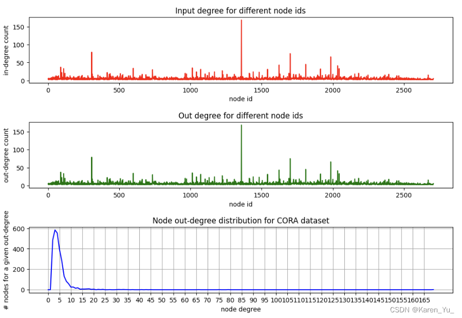
Cora结果如上图所示,可以看出:
- 上面的两张图是一样的,因为我们把Cora看作是一个无向图(尽管它自然应该被建模为一个有向图)。
- 某些节点有大量的边(中间的峰值),但大多数节点的边要少得多。
- 第三张图以直方图的形式很好地可视化了这一点——大多数节点只有2-5条边(因此最左边的峰值)。
"""
Check out this blog for available graph visualization tools:
    https://towardsdatascience.com/large-graph-visualization-tools-and-approaches-2b8758a1cd59

Basically depending on how big your graph is there may be better drawing tools than igraph.

Note: I unfortunatelly had to flatten this function since igraph is having some problems with Jupyter Notebook,
we'll only call it here so it's fine!

"""

dataset_name = config['dataset_name']
visualization_tool=GraphVisualizationTool.IGRAPH

if isinstance(edge_index, torch.Tensor):
    edge_index_np = edge_index.cpu().numpy()

if isinstance(node_labels, torch.Tensor):
    node_labels_np = node_labels.cpu().numpy()

num_of_nodes = len(node_labels_np)
edge_index_tuples = list(zip(edge_index_np[0, :], edge_index_np[1, :]))  # igraph requires this format

# Construct the igraph graph
ig_graph = ig.Graph()
ig_graph.add_vertices(num_of_nodes)
ig_graph.add_edges(edge_index_tuples)

# Prepare the visualization settings dictionary
visual_style = {}

# Defines the size of the plot and margins
# go berserk here try (3000, 3000) it looks amazing in Jupyter!!! (you'll have to adjust the vertex_size though!)
visual_style["bbox"] = (700, 700)
visual_style["margin"] = 5

# I've chosen the edge thickness such that it's proportional to the number of shortest paths (geodesics)
# that go through a certain edge in our graph (edge_betweenness function, a simple ad hoc heuristic)

# line1: I use log otherwise some edges will be too thick and others not visible at all
# edge_betweeness returns < 1 for certain edges that's why I use clip as log would be negative for those edges
# line2: Normalize so that the thickest edge is 1 otherwise edges appear too thick on the chart
# line3: The idea here is to make the strongest edge stay stronger than others, 6 just worked, don't dwell on it

edge_weights_raw = np.clip(np.log(np.asarray(ig_graph.edge_betweenness())+1e-16), a_min=0, a_max=None)
edge_weights_raw_normalized = edge_weights_raw / np.max(edge_weights_raw)
edge_weights = [w**6 for w in edge_weights_raw_normalized]
visual_style["edge_width"] = edge_weights

# A simple heuristic for vertex size. Size ~ (degree / 4) (it gave nice results I tried log and sqrt as well)
visual_style["vertex_size"] = [deg / 4 for deg in ig_graph.degree()]

# This is the only part that's Cora specific as Cora has 7 labels
if dataset_name.lower() == DatasetType.CORA.name.lower():
    visual_style["vertex_color"] = [cora_label_to_color_map[label] for label in node_labels_np]
else:
    print('Feel free to add custom color scheme for your specific dataset. Using igraph default coloring.')

# Set the layout - the way the graph is presented on a 2D chart. Graph drawing is a subfield for itself!
# I used "Kamada Kawai" a force-directed method, this family of methods are based on physical system simulation.
# (layout_drl also gave nice results for Cora)
visual_style["layout"] = ig_graph.layout_kamada_kawai()

print('Plotting results ... (it may take couple of seconds).')
ig.plot(ig_graph, **visual_style)

# This website has got some awesome visualizations check it out:
# http://networkrepository.com/graphvis.php?d=./data/gsm50/labeled/cora.edges
----------------------------------------------------------------------------------------------
OK到此为止,算是初步认识了Cora数据集,这里附上前面用来解释代码的toy dataset做可视化的流程:
# Visualization related imports
import matplotlib.pyplot as plt
import networkx as nx
import igraph as ig

# Main computation libraries
import scipy.sparse as sp
import numpy as np
import pandas as pd

# 节点特征
node_df = pd.DataFrame({
    'w_0': [1., 0., 1., 0., 1., 0., 1., 0.],
    'w_1': [0., 0., 0., 0., 1., 0., 1., 0.],
    'w_2': [1., 1., 1., 1., 1., 1., 1., 1.],
    'w_4': [0., 1., 0., 1., 1., 0., 1., 1.]
})
num_of_nodes = 8
node_df = sp.csr_matrix(node_df.values)
node_df_sum = np.array(node_df.sum(-1))
node_df_inv_sum = np.power(node_df_sum, -1).squeeze()
# 某些和可能是0,所以1/0会给我们inf,所以我们用1代替
node_df_inv_sum[np.isinf(node_df_inv_sum)] = 1.
diag_node_df_sum_matrix = sp.diags(node_df_inv_sum)
topology = diag_node_df_sum_matrix.dot(node_df).toarray()
# 边
adj_list_dict = {
    0: [1, 2, 5],
    1: [0, 2, 3, 4],
    2: [0, 1, 5],
    3: [1, 4, 5],
    4: [1, 3, 6],
    5: [0, 2, 3, 6 ,7],
    6: [4, 5, 7],
    7: [5, 6]
}

source_nodes_ids, target_nodes_ids = [], []
seen_edges = set()
for src_node, neighboring_nodes in adj_list_dict.items():
    for trg_node in neighboring_nodes:
        # if this edge hasn't been seen so far we add it to the edge index (coalescing - removing duplicates)
        if (src_node, trg_node) not in seen_edges:  # it'd be easy to explicitly remove self-edges (Cora has none..)
            source_nodes_ids.append(src_node)
            target_nodes_ids.append(trg_node)

            seen_edges.add((src_node, trg_node))
source_nodes_ids.extend(np.arange(num_of_nodes))
target_nodes_ids.extend(np.arange(num_of_nodes))
edge_index = np.row_stack((source_nodes_ids, target_nodes_ids))

in_degrees = np.zeros(num_of_nodes, dtype=np.int_)
out_degrees = np.zeros(num_of_nodes, dtype=np.int_)

num_of_edges = edge_index.shape[1]
for cnt in range(num_of_edges):
    source_node_id = edge_index[0, cnt]
    target_node_id = edge_index[1, cnt]

    out_degrees[source_node_id] += 1  # source node points towards some other node -> increment its out degree
    in_degrees[target_node_id] += 1  # similarly here

hist = np.zeros(np.max(out_degrees) + 1)
for out_degree in out_degrees:
    hist[out_degree] += 1

fig = plt.figure(figsize=(12,8), dpi=100)  # otherwise plots are really small in Jupyter Notebook
fig.subplots_adjust(hspace=0.6)

plt.subplot(311)
plt.plot(in_degrees, color='red')
plt.xlabel('node id'); plt.ylabel('in-degree count'); plt.title('Input degree for different node ids')

plt.subplot(312)
plt.plot(out_degrees, color='green')
plt.xlabel('node id'); plt.ylabel('out-degree count'); plt.title('Out degree for different node ids')

plt.subplot(313)
plt.plot(hist, color='blue')
plt.xlabel('node degree')
plt.ylabel('# nodes for a given out-degree')
plt.title(f'Node out-degree distribution for toy data dataset')
plt.xticks(np.arange(0, len(hist), 5.0))

plt.grid(True)
plt.show()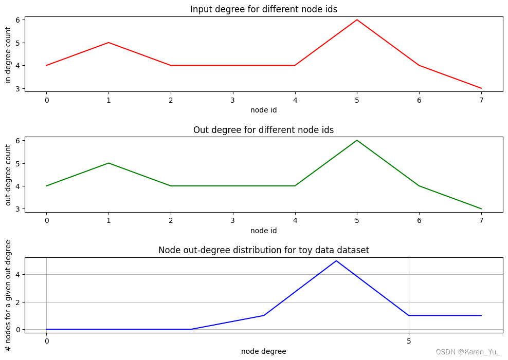
label_to_color_map = {0: "red", 1: "blue"}
edge_index = torch.from_numpy(edge_index)
node_labels = np.array([0,0,0,1,1,0,1,1])
node_labels = torch.from_numpy(node_labels)
edge_index_np = edge_index.cpu().numpy()
node_labels_np = node_labels.cpu().numpy()
print(type(node_labels), len(node_labels))
num_of_nodes = len(node_labels_np)
edge_index_tuples = list(zip(edge_index_np[0, :], edge_index_np[1, :]))

# Construct the igraph graph
ig_graph = ig.Graph()
ig_graph.add_vertices(num_of_nodes)
ig_graph.add_edges(edge_index_tuples)

# Prepare the visualization settings dictionary
visual_style = {}

# Defines the size of the plot and margins
visual_style["bbox"] = (400, 400)
visual_style["margin"] = 20

edge_weights_raw = np.clip(np.log(np.asarray(ig_graph.edge_betweenness())+1e-16), a_min=0, a_max=None)
edge_weights_raw_normalized = edge_weights_raw / np.max(edge_weights_raw)
edge_weights = [w**6 for w in edge_weights_raw_normalized]
visual_style["edge_width"] = edge_weights
visual_style["vertex_color"] = [label_to_color_map[label] for label in node_labels_np]
visual_style["layout"] = ig_graph.layout_kamada_kawai()
ig.plot(ig_graph, **visual_style)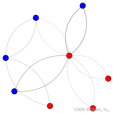


 1万+
1万+


 被折叠的 条评论
为什么被折叠?
被折叠的 条评论
为什么被折叠?
 到【灌水乐园】发言


