Logistic回归

Logistic回归

对于之前说到的线性模型$y=x\ast w+b$，y的范围是一个线性的实数域R，成为回归任务。

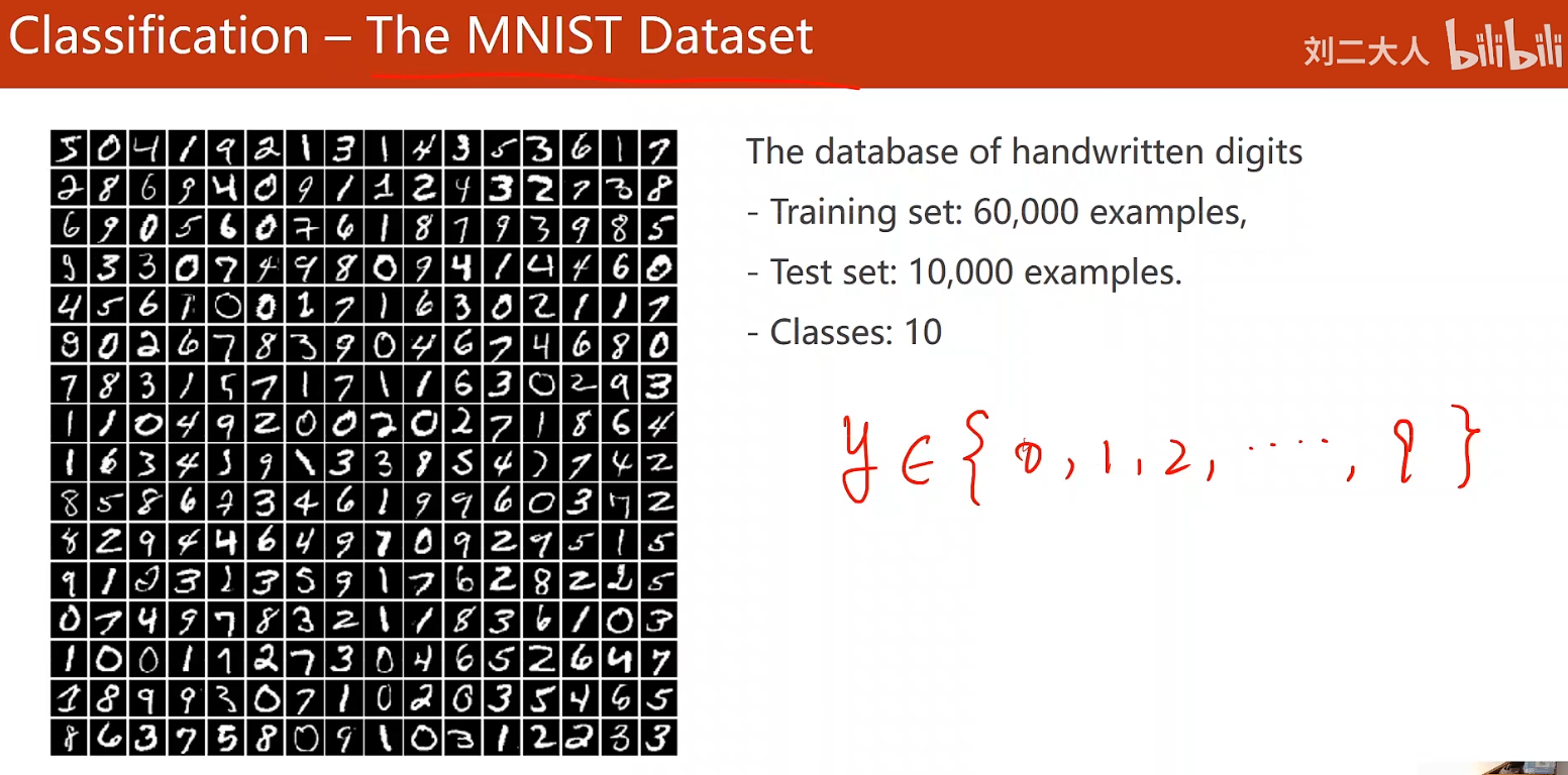
事实上机器学习中很多任务是分类任务：

首先说到两个适合练习用的数据集，

MNIST数据集，即手写体数据集，包含0-9共10个数字的手写体图片；

使用代码如下：

import torchvision
# torchvision提供下载方式，root是下载位置，train代表是否设置为训练集，download代表是否需要下载
train_set = torchvision.datasets.MNIST(root='../dataset/MNIST', train=True, download=True)
test_set = torchvision.datasets.MNIST(root='../dataset/MNIST', train=False, download=True)

CIFAR-10数据集，包含10个种类，使用方式类似。

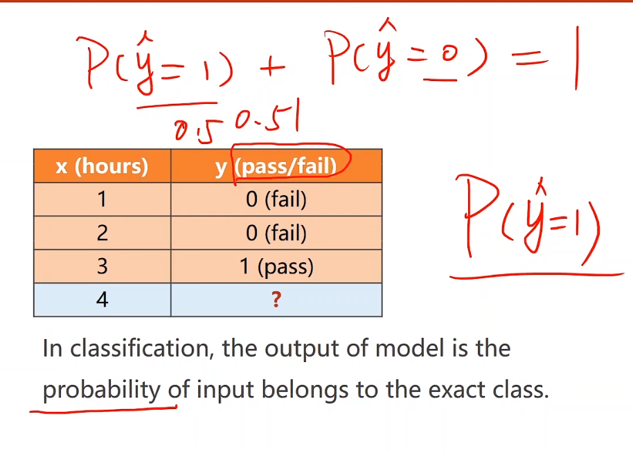
分类问题关键是要输出目标的概率

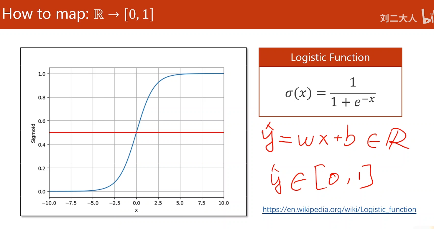
就需要使用一个Sigmoid函数将输出值限定到0-1，

此类函数有许多，其中最常用的是Logistic函数：
$$\sigma (x)=\frac{1}{1+e^{-x}}$$

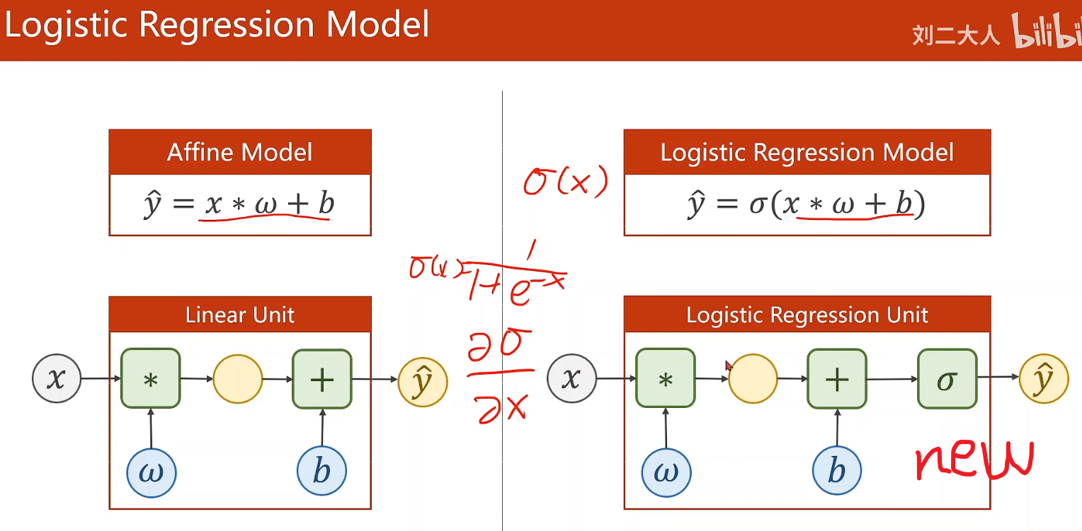
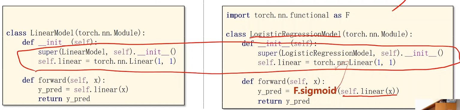
相当于就是在原来神经网络单元的最后加了一个Logistic函数

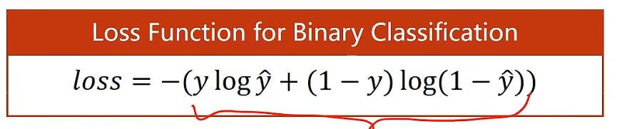
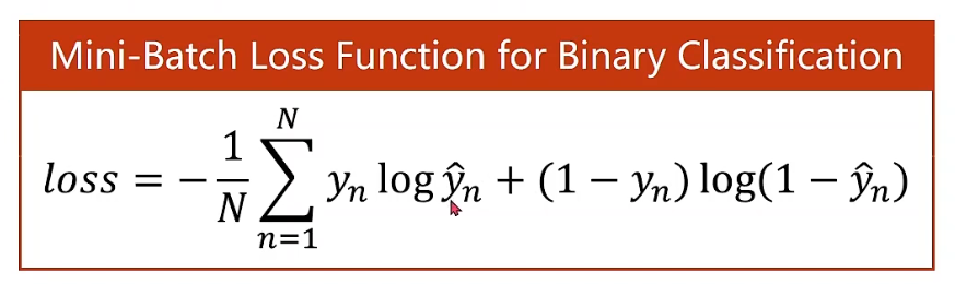
二分类任务（只有两类）中用到的损失函数BCELoss，即交叉熵损失函数：

多个样本下：

加入Logistic回归之后的Model变化：

程序

import torch
import torch.nn.functional as F

x_data = torch.Tensor([[1.0], [2.0], [3.0]])
y_data = torch.Tensor([[0], [0], [1]])

class LogisticRegressionModel(torch.nn.Module):
    def __init__(self):
        super(LogisticRegressionModel, self).__init__()
        self.linear = torch.nn.Linear(1, 1)

    def forward(self, x):
        y_pred = F.sigmoid(self.linear(x))
        return y_pred

model = LogisticRegressionModel()
criterion = torch.nn.BCELoss(size_average=False)
optimizer = torch.optim.SGD(model.parameters(), lr=0.01)

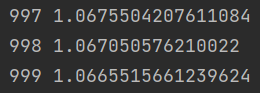
for epoch in range(1000):
    y_pred = model(x_data)
    loss = criterion(y_pred, y_data)
    print(epoch, loss.item())

    optimizer.zero_grad()
    loss.backward()
    optimizer.step()

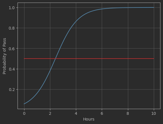
import numpy as np
import matplotlib.pyplot as plt

x = np.linspace(0, 10, 200)
x_t = torch.Tensor(x).view((200, 1))
y_t = model(x_t)
y = y_t.data.numpy()

plt.plot(x, y)
plt.plot([0, 10], [0.5, 0.5], c='r')
plt.xlabel('Hours')
plt.ylabel('Probability of Pass')
plt.grid()
plt.show()