NetSim网络仿真使用及静态路由配置

🍰 个人主页:不摆烂的小劉
🍞文章有不合理的地方请各位大佬指正。
🍉文章不定期持续更新，如果我的文章对你有帮助➡️ 关注🙏🏻 点赞👍 收藏⭐️

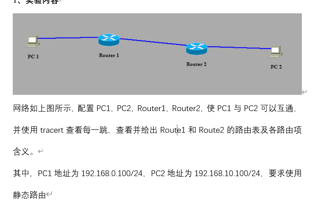
NetSim网络仿真使用及静态路由配置。

实验要求及其步骤

使用Boson NetWork Designer设计网络拓扑图

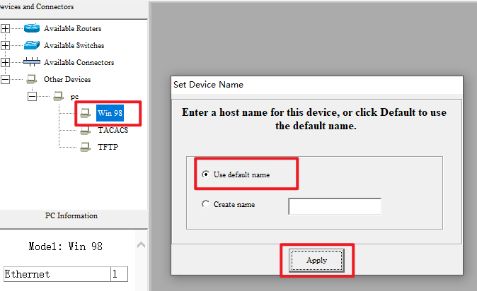
添加PC

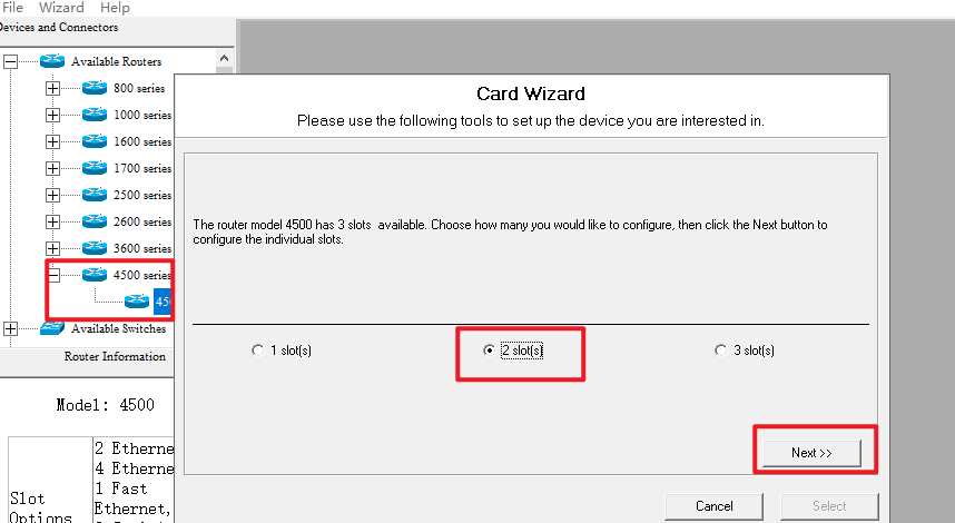
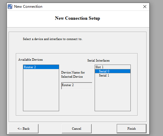
添加路由器

选择路由接口

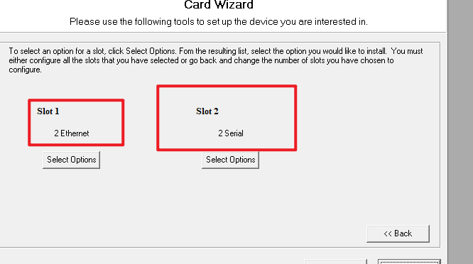
点击Select
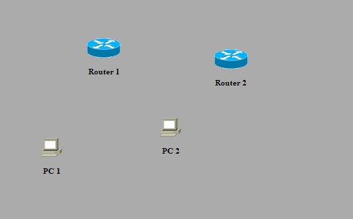
效果图

添加连接

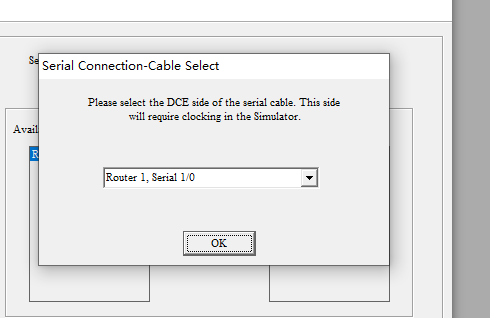
添加Serial连接

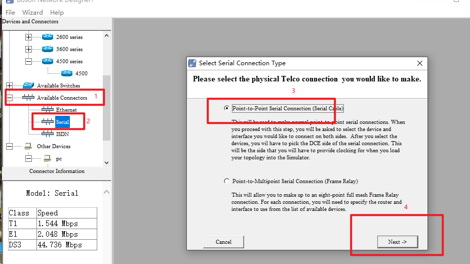
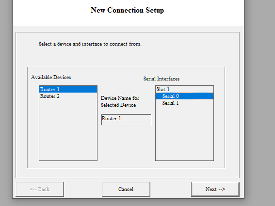
选择连接接口（选择最好和我的一样，下面会用到）

添加Ethernet连接

Router1与PC1使用Ethernet连接

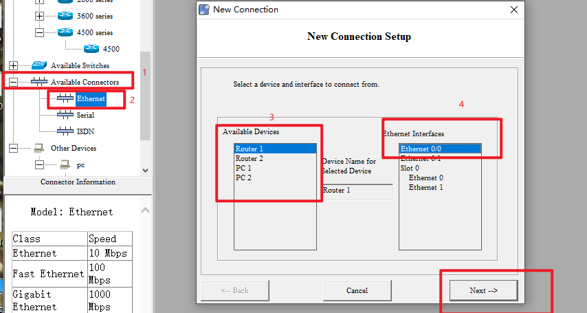
同理的Router2和PC2使用Ethernet连接起来
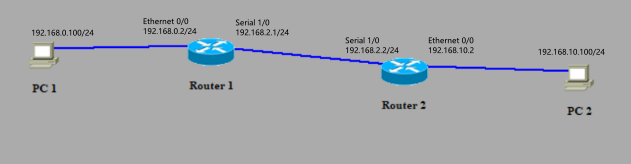
配置好如图
双击路由器Router1如图

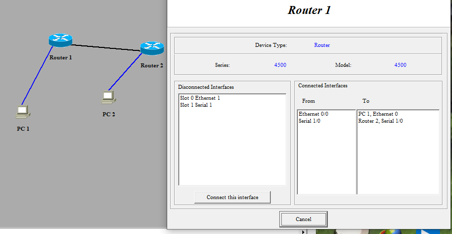
拓扑图配置完毕

配置Boson NetSim for CCNP

接下来使用Boson NetSim for CCNP完成接下来实验

配置Router1

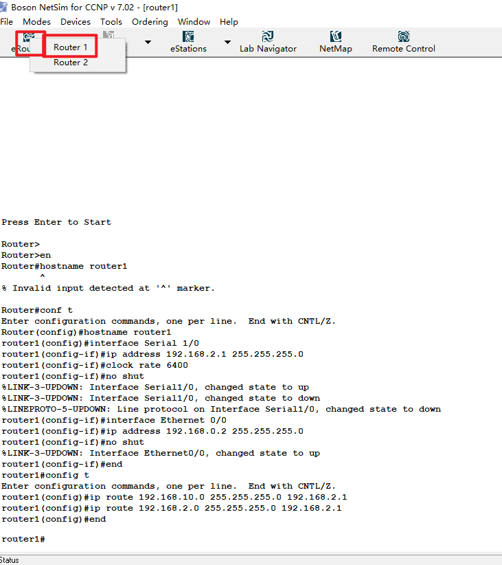
en
conf t
hostname router1
interface Serial 1/0
ip address 192.168.2.1 255.255.255.0
clock rate 6400//设置时钟频率，只在Serial 连接中配置，且只需要在这一个路由器中配置，另一个路由去里面则不用设置
no shut
interface Ethernet 0/0
ip address 192.168.0.2 255.255.255.0
no shut
end
config t
ip route 192.168.10.0 255.255.255.0 192.168.2.1//静态路由
ip route 192.168.2.0 255.255.255.0 192.168.2.1
end

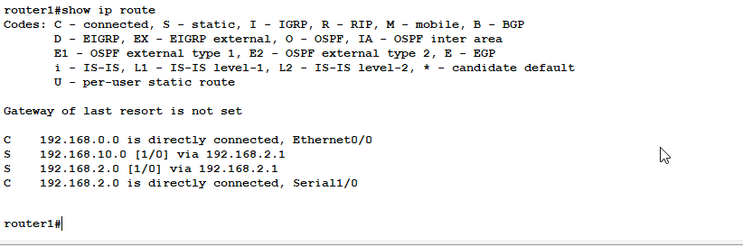
查看route1路由表

配置router2

//router2
en 
conf t
hostname router2
interface Serial 1/0
ip address 192.168.2.2 255.255.255.0
no shut
interface Ethernet 0/0
ip address 192.168.10.2 255.255.255.0
no shut
end
config t
ip route 192.168.0.0 255.255.255.0 192.168.2.2
ip route 192.168.2.0 255.255.255.0 192.168.2.2
end
ping 192.168.2.1//测试两个路由器的连通性，若出现Success rate *****（省略）则两个路由器成功建立关联

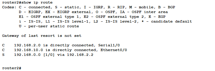
查看route2路由表

配置PC1

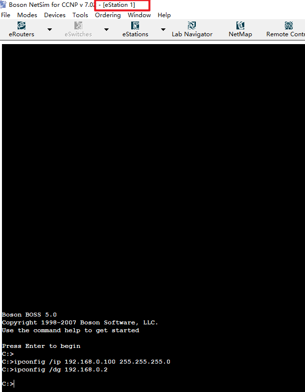
//PC1 PC1与Router1相连接，Ethernet 0/0对应的ip即为PC1的网关
//先分配ip地址，根据实验要求 PC1分配地址为192.168.0.100
ipconfig /ip 192.168.0.100 255.255.255.0
//设置网关
ipconfig /dg 192.168.0.2
//PC1已经配置好了，可以测试试一下
ping 

PC2

//PC1 PC1与Router1相连接，Ethernet 0/0对应的ip即为PC1的网关
//先分配ip地址，根据实验要求 PC1分配地址为192.168.0.100
ipconfig /ip 192.168.0.100 255.255.255.0
//设置网关
ipconfig /dg 192.168.0.2
//PC1已经配置好了，可以测试试一下
ping 

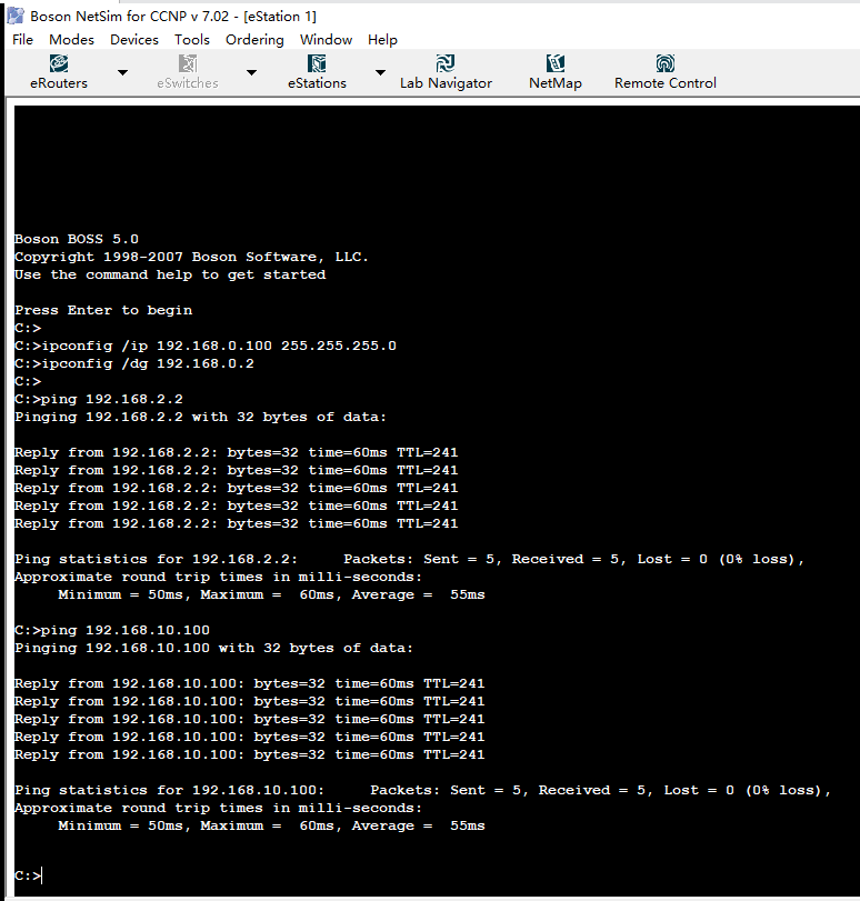
测试连通性（完成）

PC1 ping Router2和PC2

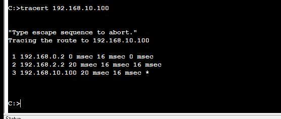
使用tracert查看ip跳转的路径

实验完成！！！！🔥🔥🔥🔥
如果对你有帮助，点个👍👍