Normalization Techniques: BN and LN

Normalization Techniques

Motivation: Why needs Normalization?

Normalization has always been an active area of research in deep learning. There are some benefits of it:

• It reduces Internal Covariate Shift. It is the change in the distribution of network activations due to the change in network parameters during training. It will move many of the distribution of network activations into the saturated regime of the nonlinearity and slow down the convergence. To improve training, we seek to reduce the internal covariate shift.
• Normalization makes loss surface smoother.
• It makes the Optimization faster because normalization doesn’t allow weights to explode all over the place and restricts them to a certain range.

Batch Normalization

Training Phase

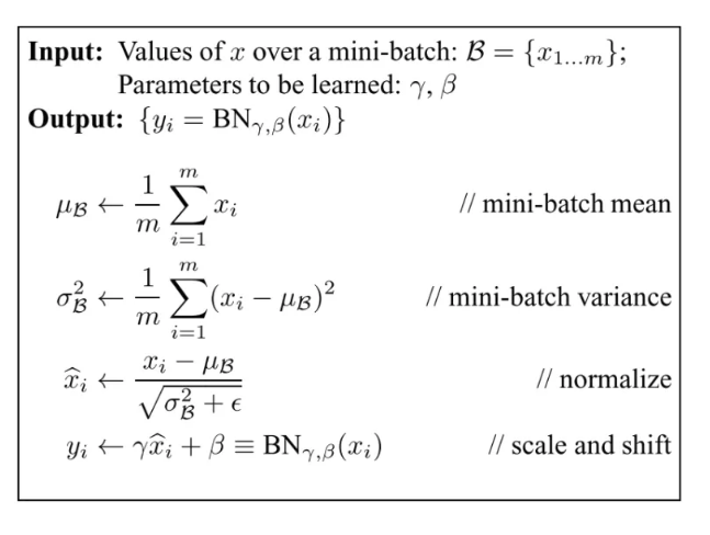
Batch normalization is a method that normalizes activations in a network across the mini-batch of definite size. For each feature, batch normalization computes the mean and variance of that feature in the mini-batch . It then substracts the mean and divides the feature by its mini-batch standard deviation.

However, simply normalizing each input of a layer may change what the layer can represent. For instance, normalizing the inputs of a sigmoid would constrain them to the linear regime of the nonlinearity. To address this and make sure the transformation inserted in the network can represent the identity transform, a pair of parameters ${\gamma }^{(k)},{\beta }^{(k)}$ where introduced to scale and shift the normalized value for each activation $x^{(k)}$:
$$y^{(k)}={\gamma }^{(k)}{\hat{x}}^{(k)}+{\beta }^{(k)}$$
These parameters are learned along with the original model parameters, and restore the representation power of the network. Indeed, by setting ${\gamma }^{(k)}=\sqrt{Var[x^{(k)}]}$ and ${\beta }^{(k)}=E[x^{(k)}]$, we could recover the original activatioins, if that were the optimal thing to do.

The batch normalization can be summarized as:

Inference Phase

During the inference phase, specifically when you only have one test sample, doing batch normalization as the one in training phase does not make sense, because your outputs at each layer of the network will be exactly zero. Instead. we use running mean and running variance calculated during training.

At each time step $t$ during training, the runing mean ${\mu }_B^{\prime }[t]$ and running variance ${\sigma }_B^{\prime 2}$ are calculated as:
$${\mu }_B^{}$$