机器学习笔记之~感受野receptive field

在卷积神经网络中，receptive field是一个重要的概念，对它的理解，也是理解卷积神经网络的一个重要方面。

从直观上来讲，receptive field是卷积神经网络中某一层输出结果中的一个像素点对应的输入层的一个映射。这里对输入层的理解分为两种讨观点，一种认为是本层所对应的输入图，另一种认为是原始图像。个人观点应该是对应的输入图，而不是原始图像。

 

下面这篇是原文：

https://medium.com/mlreview/a-guide-to-receptive-field-arithmetic-for-convolutional-neural-networks-e0f514068807

A guide to receptive field arithmetic for Convolutional Neural Networks

The receptive field is perhaps one of the most important concepts in Convolutional Neural Networks (CNNs) that deserves more attention from the literature. All of the state-of-the-art object recognition methods design their model architectures around this idea. However, to my best knowledge, currently there is no complete guide on how to calculate and visualize the receptive field information of a CNN. This post fills in the gap by introducing a new way to visualize feature maps in a CNN that exposes the receptive field information, accompanied by a complete receptive field calculation that can be used for any CNN architecture. I’ve also implemented a simple program to demonstrate the calculation so that anyone can start computing the receptive field and gain better knowledge about the CNN architecture that they are working with.

To follow this post, I assume that you are familiar with the CNN concept, especially the convolutional and pooling operations. You can refresh your CNN knowledge by going through the paper “A guide to convolution arithmetic for deep learning [1]”. It will not take you more than half an hour if you have some prior knowledge about CNNs. This post is in fact inspired by that paper and uses similar notations.

Note: If you want to learn more about how CNNs can be used for Object Recognition, this post is for you.

 

The fixed-sized CNN feature map visualization

The receptive field is defined as the region in the input space that a particular CNN’s feature is looking at (i.e. be affected by). A receptive field of a feature can be described by its center location and its size. (Edit later) However, not all pixels in a receptive field is equally important to its corresponding CNN’s feature. Within a receptive field, the closer a pixel to the center of the field, the more it contributes to the calculation of the output feature. Which means that a feature does not only look at a particular region (i.e. its receptive field) in the input image, but also focus exponentially more to the middle of that region. This important insight will be explained further in another blog post. For now, we focus on calculating the location and size of a particular receptive field.

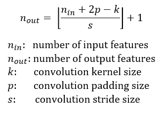
Figure 1 shows some receptive field examples. By applying a convolution C with kernel size k = 3x3, padding size p = 1x1, stride s = 2x2 on an input map 5x5, we will get an output feature map 3x3 (green map). Applying the same convolution on top of the 3x3 feature map, we will get a 2x2 feature map (orange map). The number of output features in each dimension can be calculated using the following formula, which is explained in detail in [1].

Note that in this post, to simplify things, I assume the CNN architecture to be symmetric, and the input image to be square. So both dimensions have the same values for all variables. If the CNN architecture or the input image is asymmetric, you can calculate the feature map attributes separately for each dimension.

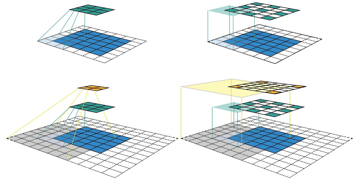
Figure 1: Two ways to visualize CNN feature maps. In all cases, we uses the convolution C with kernel size k = 3x3, padding size p = 1x1, stride s = 2x2. (Top row) Applying the convolution on a 5x5 input map to produce the 3x3 green feature map. (Bottom row) Applying the same convolution on top of the green feature map to produce the 2x2 orange feature map. (Left column) The common way to visualize a CNN feature map. Only looking at the feature map, we do not know where a feature is looking at (the center location of its receptive field) and how big is that region (its receptive field size). It will be impossible to keep track of the receptive field information in a deep CNN. (Right column) The fixed-sized CNN feature map visualization, where the size of each feature map is fixed, and the feature is located at the center of its receptive field.

The left column of Figure 1 shows a common way to visualize a CNN feature map. In that visualization, although by looking at a feature map, we know how many features it contains. It is impossible to know where each feature is looking at (the center location of its receptive field) and how big is that region (its receptive field size). The right column of Figure 1 shows the fixed-sized CNN visualization, which solves the problem by keeping the size of all feature maps constant and equal to the input map. Each feature is then marked at the center of its receptive field location. Because all features in a feature map have the same receptive field size, we can simply draw a bounding box around one feature to represent its receptive field size. We don’t have to map this bounding box all the way down to the input layer since the feature map is already represented in the same size of the input layer. Figure 2 shows another example using the same convolution but applied on a bigger input map — 7x7. We can either plot the fixed-sized CNN feature maps in 3D (Left) or in 2D (Right). Notice that the size of the receptive field in Figure 2 escalates very quickly to the point that the receptive field of the center feature of the second feature layer covers almost the whole input map. This is an important insight which was used to improve the design of a deep CNN.

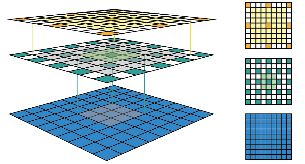
Figure 2: Another fixed-sized CNN feature map representation. The same convolution C is applied on a bigger input map with i = 7x7. I drew the receptive field bounding box around the center feature and removed the padding grid for a clearer view. The fixed-sized CNN feature map can be presented in 3D (Left) or 2D (Right).

 

Receptive Field Arithmetic

To calculate the receptive field in each layer, besides the number of features nin each dimension, we need to keep track of some extra information for each layer. These include the current receptive field size r , the distance between two adjacent features (or jump) j, and the center coordinate of the upper left feature (the first feature) start. Note that the center coordinate of a feature is defined to be the center coordinate of its receptive field, as shown in the fixed-sized CNN feature map above. When applying a convolution with the kernel size k, the padding size p, and the stride size s, the attributes of the output layer can be calculated by the following equations:

• The first equation calculates the number of output features based on the number of input features and the convolution properties. This is the same equation presented in [1].
• The second equation calculates the jump in the output feature map, which is equal to the jump in the input map times the number of input features that you jump over when applying the convolution (the stride size).
• The third equation calculates the receptive field size of the output feature map, which is equal to the area that covered by k input features (k-1)*j_inplus the extra area that covered by the receptive field of the input feature that on the border.
• The fourth equation calculates the center position of the receptive field of the first output feature, which is equal to the center position of the first input feature plus the distance from the location of the first input feature to the center of the first convolution (k-1)/2*j_in minus the padding spacep*j_in. Note that we need to multiply with the jump of the input feature map in both cases to get the actual distance/space.

The first layer is the input layer, which always has n = image size, r = 1, j = 1, and start = 0.5. Note that in Figure 3, I used the coordinate system in which the center of the first feature of the input layer is at 0.5. By applying the four above equations recursively, we can calculate the receptive field information for all feature maps in a CNN. Figure 3 shows an example of how these equations work.

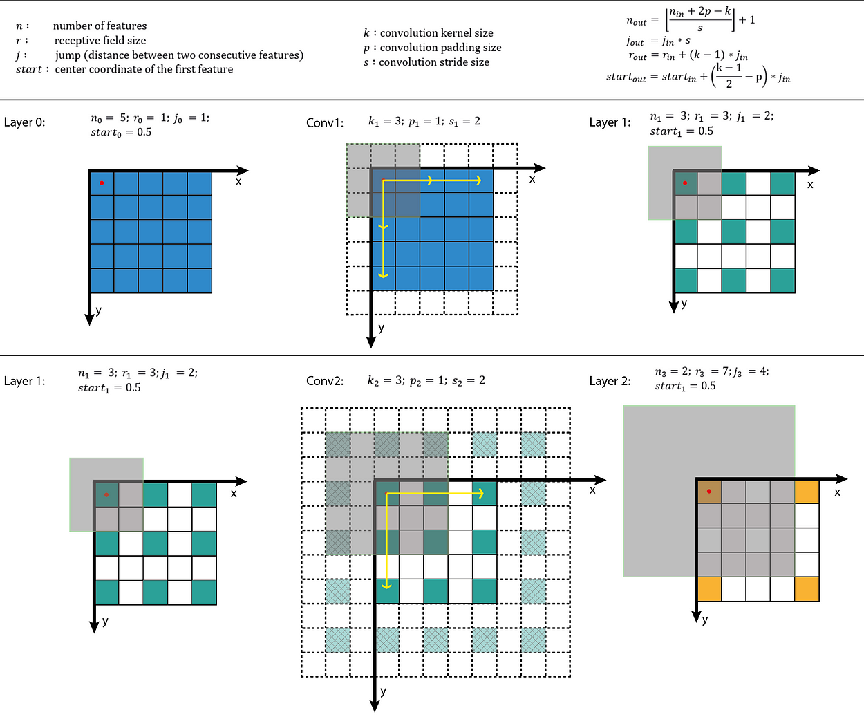
Figure 3: Applying the receptive field calculation on the example given in Figure 1. The first row shows the notations and general equations, while the second and the last row shows the process of applying it to calculate the receptive field of the output layer given the input layer information.

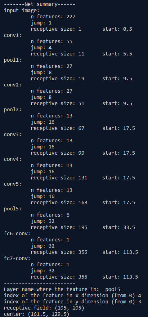
I’ve also created a small python program that calculates the receptive field information for all layers in a given CNN architecture. It also allows you to input the name of any feature map and the index of a feature in that map, and returns the size and location of the corresponding receptive field. The following figure shows an output example when we use the AlexNet. The code is provided at the end of this post.

# [filter size, stride, padding]
#Assume the two dimensions are the same
#Each kernel requires the following parameters:
# - k_i: kernel size
# - s_i: stride
# - p_i: padding (if padding is uneven, right padding will higher than left padding; "SAME" option in tensorflow)
# 
#Each layer i requires the following parameters to be fully represented: 
# - n_i: number of feature (data layer has n_1 = imagesize )
# - j_i: distance (projected to image pixel distance) between center of two adjacent features
# - r_i: receptive field of a feature in layer i
# - start_i: position of the first feature's receptive field in layer i (idx start from 0, negative means the center fall into padding)

import math
convnet =   [[11,4,0],[3,2,0],[5,1,2],[3,2,0],[3,1,1],[3,1,1],[3,1,1],[3,2,0],[6,1,0], [1, 1, 0]]
layer_names = ['conv1','pool1','conv2','pool2','conv3','conv4','conv5','pool5','fc6-conv', 'fc7-conv']
imsize = 227

def outFromIn(conv, layerIn):
  n_in = layerIn[0]
  j_in = layerIn[1]
  r_in = layerIn[2]
  start_in = layerIn[3]
  k = conv[0]
  s = conv[1]
  p = conv[2]
  
  n_out = math.floor((n_in - k + 2*p)/s) + 1
  actualP = (n_out-1)*s - n_in + k 
  pR = math.ceil(actualP/2)
  pL = math.floor(actualP/2)
  
  j_out = j_in * s
  r_out = r_in + (k - 1)*j_in
  start_out = start_in + ((k-1)/2 - pL)*j_in
  return n_out, j_out, r_out, start_out
  
def printLayer(layer, layer_name):
  print(layer_name + ":")
  print("\t n features: %s \n \t jump: %s \n \t receptive size: %s \t start: %s " % (layer[0], layer[1], layer[2], layer[3]))
 
layerInfos = []
if __name__ == '__main__':
#first layer is the data layer (image) with n_0 = image size; j_0 = 1; r_0 = 1; and start_0 = 0.5
  print ("-------Net summary------")
  currentLayer = [imsize, 1, 1, 0.5]
  printLayer(currentLayer, "input image")
  for i in range(len(convnet)):
    currentLayer = outFromIn(convnet[i], currentLayer)
    layerInfos.append(currentLayer)
    printLayer(currentLayer, layer_names[i])
  print ("------------------------")
  layer_name = raw_input ("Layer name where the feature in: ")
  layer_idx = layer_names.index(layer_name)
  idx_x = int(raw_input ("index of the feature in x dimension (from 0)"))
  idx_y = int(raw_input ("index of the feature in y dimension (from 0)"))
  
  n = layerInfos[layer_idx][0]
  j = layerInfos[layer_idx][1]
  r = layerInfos[layer_idx][2]
  start = layerInfos[layer_idx][3]
  assert(idx_x < n)
  assert(idx_y < n)
  
  print ("receptive field: (%s, %s)" % (r, r))
  print ("center: (%s, %s)" % (start+idx_x*j, start+idx_y*j))

个人对receptive field的理解处于初步阶段，欢迎大家交流。

感谢原文作者分享的receptive field理论，很全面也很有助于理解

另外提供两篇关于receptive field的不错的博文：

1. https://blog.csdn.net/u010725283/article/details/78593410

2. https://zhuanlan.zhihu.com/p/26663577