t2_Working W DataInTableau_format_extract_refresh_OLTP_OLAP_twb_tds_tde_hyper_tbm_tps_tds_tms_Filter

Tableau offers the ability to connect to nearly any data source. It does so using a unique paradigm[ˈpærədaɪm]范例,样板,范式 that allows it to leverage the power and efficiency of existing database engines with an option to extract data locally. This chapter focuses on essential concepts of how Tableau works with data, including the following topics:

• The Tableau paradigm
• Connecting to data
• Working with extracts instead of live connections
• Tableau file types
• Metadata and sharing connections
• Joins and blends
• Filtering data

The Tableau paradigm

     The unique and exciting experience of working with data in Tableau is a result of (VizQL Visual Query Language). 

     VizQL was developed as a Stanford research project, focusing on the natural ways that humans visually perceive[pərˈsiːv]感知,理解,察觉,意识到 the world and how that could be applied to data visualization. We naturally perceive differences in size, shape, spatial location, and color. VizQL allows Tableau to translate your actions, as you drag and drop fields of data in a visual environment, into a query language that defines how the data encodes those visual elements. You will never need to read, write, or debug VizQL. As you drag and drop fields onto various shelves defining size, color, shape, and spatial location, Tableau will generate the VizQL behind the scenes. This allows you to focus on visualizing data, not writing code!

     One of the benefits of VizQL is that it provides a common way of describing how the arrangement of various fields in a view defines a query related to the data. This common baseline can then be translated into numerous flavors of SQL, MDX, and TQL (short for Tableau Query Language, used for extracted data). Tableau will automatically perform the translation of VizQL into a native query to be run by the source data engine.

     In its simplest form, the Tableau paradigm of working with data looks like the following diagram: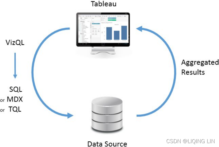

A simple example

     Go ahead and open the Chapter 02 Starter.twbx workbook located in the \LearningTableau\Chapter 02 directory and navigate to the Tableau Paradigm sheet. Take a look at the following screenshot, which was created by dropping the Region dimension on Columns and the Sales measure on Rows: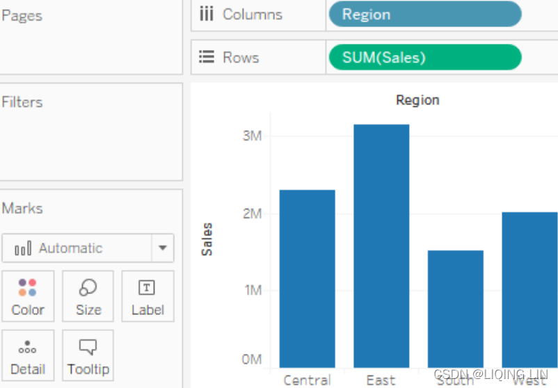

     The Region field is used as a discrete (blue) field in the view, and so defines column headers. As a dimension, it defines the level of detail in the view and slices the measure such that you get one bar per region. The Sales field is a measure aggregated by summing each sale within each region. As a continuous (green) field, Sales defines an axis.

     For the purpose of this example (although the principal is applicable to any data source), let's say you were connected live to a SQL Server database with the Superstore data stored in a table. When you first create the preceding screenshot, Tableau generates a VizQL script, which is translated into SQL script and sent to the SQL Server. The SQL Server database engine evaluates the query and returns aggregated results to Tableau, which are then rendered visually. The entire process would look something like the following diagram in Tableau's paradigm: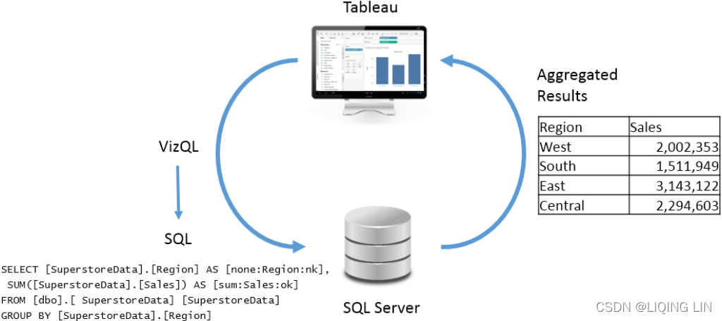

     There may have been hundreds, thousands, or even millions of rows of sales data in SQL Server. However, when SQL Server processes the query it returns aggregate results. In this case, SQL Server returns only four aggregate rows of data to Tableau—one row for each region.

     To see the aggregate data that Tableau used to draw the view,

• press Ctrl + A to select all the bars, and
• then right-click one of them and select View Data.
  

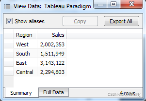
     The View Data screen allows you to observe the data in the view. The Summary tab displays the aggregate-level data that was used to render the view. The Sales values here are the sum of sales for each region. When you click the Full Data OR Underlying tab, Tableau will query the data source to retrieve all the records that make up the aggregate records. In this case, there are 9,426 underlying records, as indicated on the status bar in the lower-right corner of the following screenshot: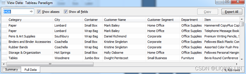

     Tableau did not need 9,426 records to draw the view, and did not request them from the data source until the Full Data OR Underlying tab was clicked.

     Database engines are optimized to perform aggregations on data. Typically, these database engines are also located on powerful servers. Tableau leverages the optimization and power of the underlying data source. In this way, Tableau can visualize massive datasets with relatively little local processing of the data.

     Additionally, Tableau will only query the data source when you make changes requiring a new query or a view refresh. Otherwise, it will use the aggregate results stored in a local cache(on the right in the figure below), as illustrated here: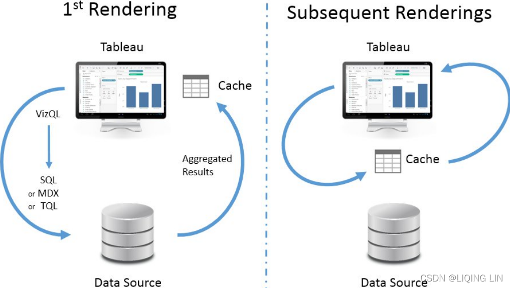

     In the preceding example, the query based on the fields in the view (that is, region as a dimension and the sum of sales as a measure) will only be issued once to the data source. When the four rows of aggregate results are returned, they are stored in the cache. Then, if you were to move Region to another visual encoding shelf, such as color, or Sales to a different visual encoding shelf, such as size, then Tableau will retrieve the aggregate rows from the cache and simply re-render the view.

     You can force Tableau to bypass the cache绕过缓存 and refresh the data from a data source by pressing F5, or selecting your data source from the Data menu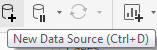 and selecting Refresh. Do this any time you want a view to reflect the most recent changes in a live data source.

     Of course, if you were to introduce new fields into the view that did not have cached results, then Tableau would send a new query to the data source, retrieve the aggregate results, and add those results to the cache.

     On occasion, a database administrator may want to find out what scripts are running against a certain database to debug performance issues, or to determine more efficient indexing or data structures. Many databases supply profiling[ˈproʊfaɪlɪŋ]（有关人或事物的）资料收集，剖析研究  utilities or log execution of queries. In addition, you can find SQL or MDX generated by Tableau in the Logs located in the My Tableau RepositoryLogs directory(C:\Users\LlQ\Documents\My Tableau Repository\Logs).

     You may also use Tableau's built-in Performance Recorder to locate the queries that have been executed. From the top menu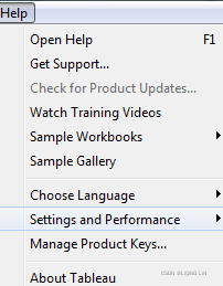, select Help | Settings and Performance | Start Performance Recording, then interact with a view, and, finally, stop the recording from the menu. Tableau will open a dashboard that will allow you to see tasks, performance, and queries that were executed during the recording session.

Connecting to data 

     There is virtually no limit to the data that Tableau can visualize! Almost every new version of Tableau adds new native connections. Tableau continues to add native connectors for cloud-based data. The web data connector allows you to write a connector for any online data you wish to retrieve. Additionally, for any database without a native connection, Tableau gives you the ability to use a generic ODBC connection. The Extract API allows you to programmatically extract and combine any data sources for use in Tableau. 

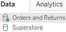
     You may have multiple data source connections to different sources in the same workbook. Each connection will show up under the Data tab on the left sidebar.

     This section will focus on a few practical examples of connecting to various data sources. We won't cover every possible connection, but will cover several that are representative of others. You may or may not have access to some of the data sources in the following examples. Don't worry if you aren't able to follow each example. Merely observe the differences. 

Connecting to data in a file

     File-based data includes all sources of data where the data is stored in a file. File-based data sources include the following:

• Extracts: A .hyper or .tde file containing data that was extracted from an original source.
• Microsoft Access: An .mdb or .accdb database file created in Access.
• Microsoft Excel: An .xls , .xlsx , or .xlsm spreadsheet created in Excel.
  Multiple Excel sheets or sub-tables may be joined or unioned together in a single connection.
• Text file: A delimited分隔的 text file, most commonly .txt , .csv , or .tab . Multiple text files in a single directory may be joined or unioned together in a single connection.
• Local cube file: A .cub file that contains multi-dimensional data. These files are typically exported from OLAP(online analytical processing) databases. 
  • Online transaction processing (OLTP) captures, stores, and processes data from transactions in real time. 
  • Online analytical processing (OLAP) uses complex queries to analyze aggregated historical data from OLTP systems
• Adobe PDF: A .pdf file that may contain tables of data that can be parsed by Tableau.
• Spatial file: A .kml , .shp , .tab , .mif , or .geojson file that contains spatial objects that can be rendered by Tableau.
• Statistical file: An .sav , .sas7bdat , .rda , or .rdata file generated by statistical tools, such as SAS or R.
• JSON file: A .json file that contains data in JSON format. 

     In addition to those mentioned previously, you can connect to Tableau files to import connections that you have saved in another Tableau workbook ( .twb or .twbx ). The connection will be imported and changes will only affect the current workbook. 

Follow this example to see a connection to an Excel file:

• 1. Navigate to the Connect to Excel sheet in the Chapter 02 Starter.twbx workbook.
• 2. From the menu, select Data | New data source and select Excel from the list of possible connections.

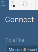
• 3. In the open dialogue, open the Superstore.xlsx file from the \Learning Tableau\Chapter 02 directory. 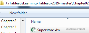Tableau will open the Data Source screen. You should see the two sheets of the Excel document listed on the left.
• 4. Double-click the Orders sheet and then the Returns sheet. Your data source screen should look similar to the following screenshot:
  

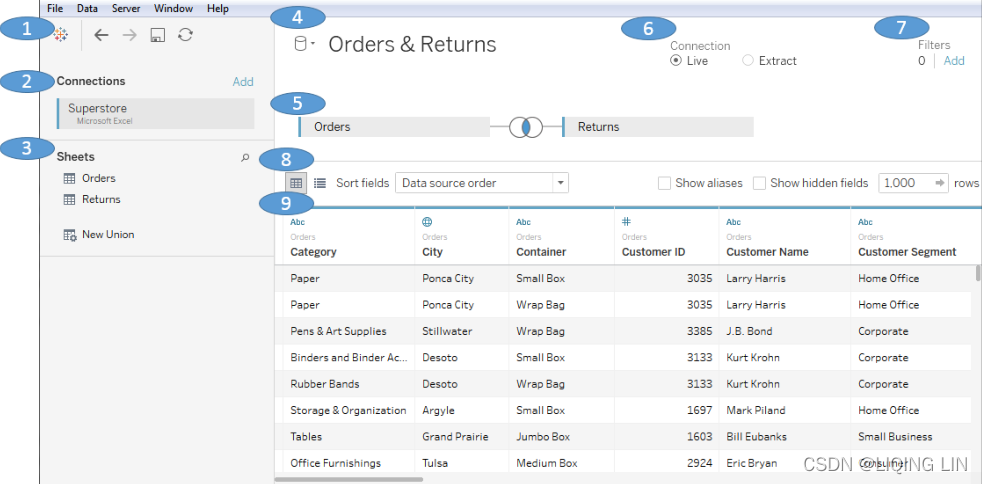
     Take some time to familiarize yourself with the Data Source screen interface, which has the following features (numbered in the preceding screenshot):

• 1. Toolbar: The toolbar has a few of the familiar controls, including undo, redo, and save. It also includes the option to refresh the current data source.
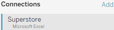
• 2. Connections: All the connections in the current data source. Click Add to add a new connection to the current data source. This allows you to join data across different connection types. Each connection will be color-coded so that you can distinguish what data is coming from which connection.
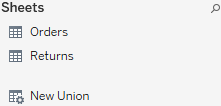
• 3. Sheets (or Tables): This lists all the tables of data available for a given connection. This includes sheets, sub-tables, and named ranges for Excel; tables, views, and stored procedures for relational databases; and other connection-dependent options, such as New Union or Custom SQL.
• 4. Data Source Name: This is the name of the currently selected data source. You may select a different data source using the drop-down arrow next to the database icon. You may click the name of the data source to edit it.
• 5. Connection Editor: Drop sheets and tables from the left into this area to make them part of the connection. For many connections, you may add multiple tables that will be joined or unioned together. We'll take a look at some advanced examples of options later in the chapter. For now, notice that you can hover over tables in this space and get options via a drop-down menu.
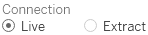
• 6. Live or Extract Options: For many data sources, you may choose whether you would like to have a live connection or an extracted connection. We'll look at these in further detail later in the chapter.
• 7. Data Source Filters: You may add filters to the data source. These will be applied at the data-source level, and thus to all views of the data using this data source in the workbook.
• 8. Preview Pane Options: These options allow you to specify whether you'd like to see a preview of the data or a list of metadata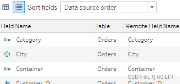, and how you would like to preview the data (examples include alias values, hidden fields shown, and how many rows you'd like to preview).
• 9. Preview Pane/Metadata View: Depending on your selection in the options, this space either displays a preview of data or a list of all fields with additional metadata. Notice that these views give you a wide array of options, such as changing data types, hiding or renaming fields, and applying various data transformation functions. We'll consider some of these options in this and later chapters.

     Once you have created and configured your data source, you may click any sheet to start using it.

Conclude this exercise with the following steps: 

• 1. Click the data source name to edit the text and rename the data source to Orders and Returns.
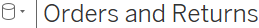
• 2. Navigate to the Connect to Excel sheet and, using the Orders and Returns data source, create a time series showing Number of Records by Return Reason. Your view should look like the following screenshot: 
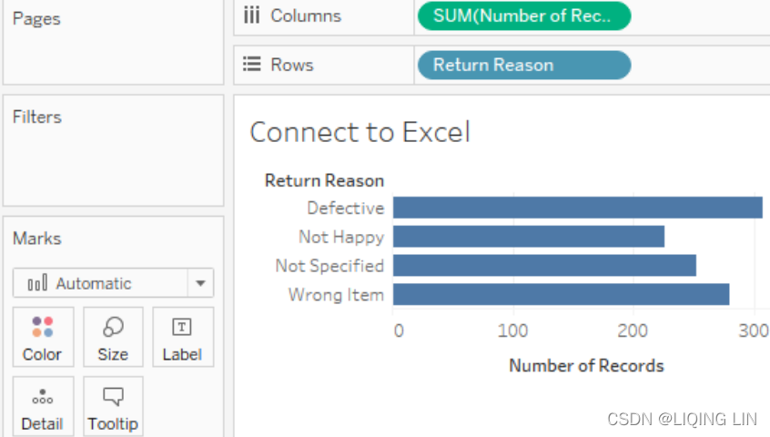
• 3. As the connection you created is based on an inner join of Orders and Returns, this view shows the number of returns for each reason code.

     If you need to edit the connection at any time,

• select Data from the menu, locate your connection, and then select Edit Data Source....
• Alternately, you may right-click any data source under the Data tab on the left sidebar and select Edit Data Source...,
• or click the Data Source tab in the lower-left. You may access the data source screen at any time by clicking the Data Source tab in the lower-left corner of Tableau Desktop. 

Connecting to data on a server

     Database servers, such as SQL Server, MySQL, Vertica, and Oracle, host data on one or more server machines and use powerful database engines to store, aggregate, sort, and serve data based on queries from client applications. Tableau can leverage the capabilities of these servers to retrieve data for visualization and analysis. Alternately, data can be extracted from these sources and stored in an extract ( .hyper or .tde ). 

     As an example of connecting to a server data source, we'll demonstrate connecting to SQL Server. If you have access to a server-based data source, you may wish to create a new data source and explore the details. However, there is no specific example to follow in the workbook in this chapter. As soon as the Microsoft SQL Server connection is selected, the interface displays options for some initial configuration as follows:

 
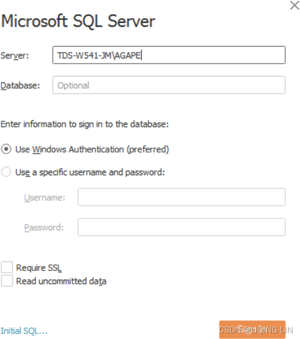
     A connection to SQL Server requires the Server name, as well as authentication information.

     A database administrator can configure SQL Server to use

• Windows Authentication or
• a SQL Server username and password.

With SQL Server, you can also optionally allow for reading uncommitted data未提交的数据. This can potentially improve performance, but may also lead to unpredictable results if data is being inserted, updated, or deleted at the same time Tableau is querying. Additionally, you may specify SQL to be run at connect time using the Initial SQL... link in the lower-left corner.

     In order to maintain high standards of security, Tableau will not save a password as part of a data source connection. This means that if you share a workbook using a live connection with someone else, they will need to have credentials to access the data. This also means that when you first open the workbook, you will need to re-enter your password for any connections requiring a password.

     Once you click the orange Sign In button, you will see a screen that is very similar to the connection screen you saw for Excel. The main difference is on the left, where you have an option for selecting a database, as shown in the following screenshot: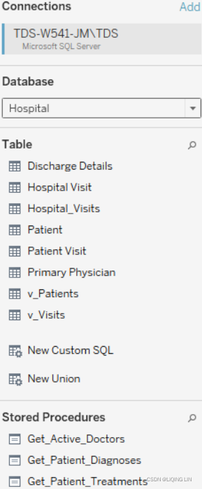 

Once you've selected a database, you will see the following:

• Table: This shows any data tables or views contained in the selected database.
• New Custom SQL: You may write your own custom SQL scripts and add them as tables. You may join these as you would any other table or view.
• New Union: You may union together tables in the database. Tableau will match fields based on name and data type, and you may additionally merge fields as needed.
• Stored Procedures: You may use a stored procedure that returns a table of data. You will be given the option of setting values for stored procedure parameters, or using or creating a Tableau parameter to pass values.

     Once you have finished configuring the connection, click a tab for any sheet to begin visualizing the data.

Connecting to data in the cloud

     Certain data connections are made to data that is hosted in the cloud. These include Amazon Redshift, Google Analytics, Google Sheets, Salesforce, and many others. It is beyond the scope of this book to cover each connection in depth, but as an example of a cloud data source, we'll consider connecting to Google Sheets.

     Google Sheets allows users to create and maintain spreadsheets of data online. Sheets may be shared and collaborated[kəˈlæbəreɪtɪd]协作,合作 on by many different users. Here, we'll walk through an example of connecting to a sheet that is shared via link.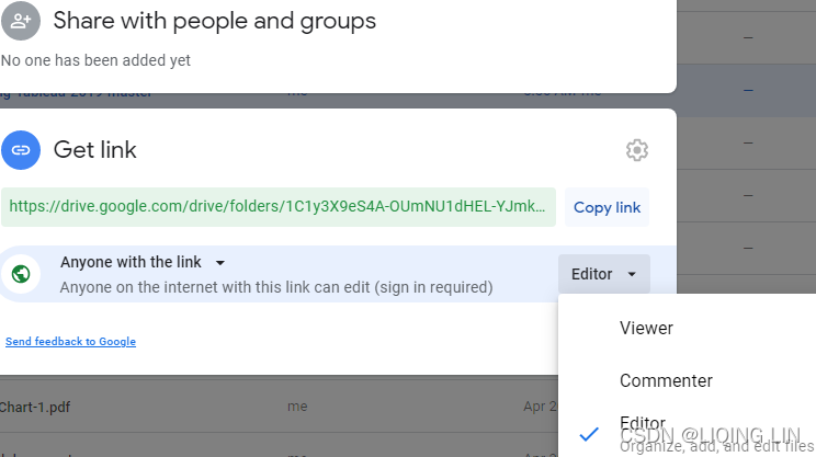

==>

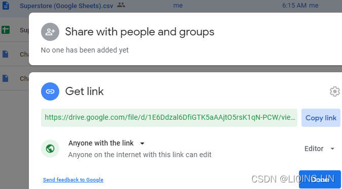
https://docs.google.com/spreadsheets/d/1F350JXCThZZvAy1FMZZkkcjWiZ81hk3HjFAk3ZyroA0/edit?usp=sharing 

     To follow the example, you'll need a free Google account. With your credentials, follow these steps:

• 1. Click the New Data Source button on the toolbar, as shown here: 
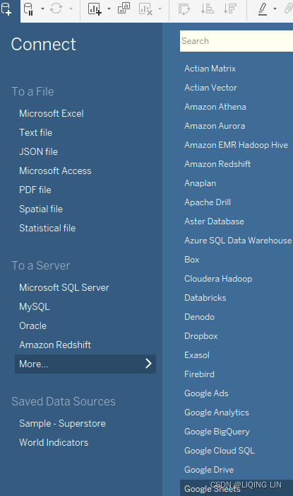
• 2. Select Google Sheets from the list of possible data sources. You may use the search box to quickly narrow the list.
  ==>
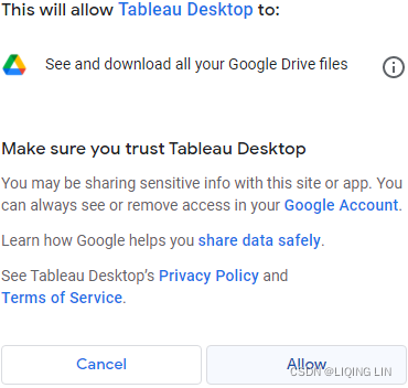
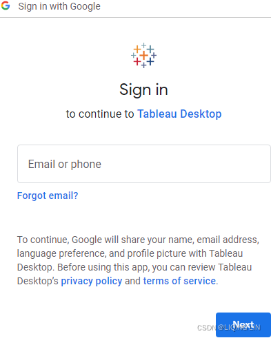
• 3. On the next screens, sign into your Google Account and allow Tableau Desktop the appropriate permissions. You will then be presented with a list of all your Google Sheets, along with preview and search capabilities, as shown in the following screenshot:
  
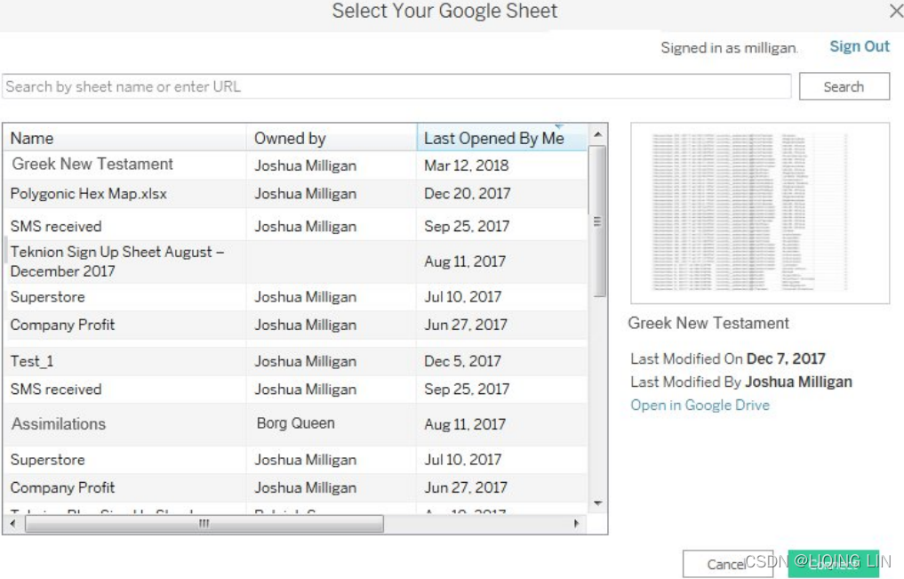
• 4. Enter this URL (for convenience, it is included in the Chapter 02 Starter workbook in the Connect to Google Sheets tab, and may be copied and pasted) into the search box and click the Search button: https://docs.google.com/spreadsheets/d/1F350JXCThZZvAy1FMZZkkcjWiZ81hk3HjFAk3ZyroA0/edit?usp=sharing .
• 5. Select the resulting Superstore sheet in the list and then click the Connect button. You should now see the Data Source screen.
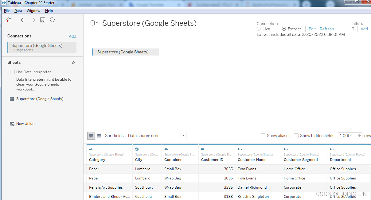
• 6. Rename the data source to Superstore (Google Sheets) . 
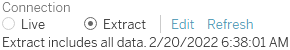
• 7. For the purpose of this example, switch the connection option from Live to Extract. When connecting to your own Google Sheets data, you may choose either Live or Extract.
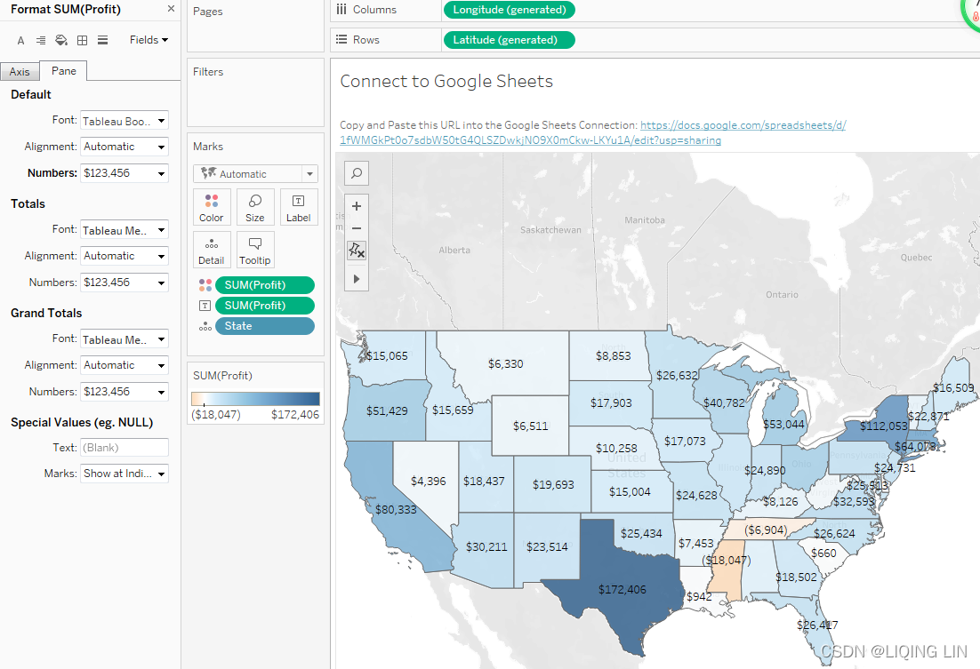
• 8. Navigate to the Connect to Google Sheets sheet. The data should be extracted within a few seconds.
• 9. Create a filled map of Profit by State, with Profit defining the Color and the Label.
• 10. Right-click the Profit field in the data pane and select Default Properties | Number Format....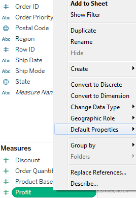The resulting dialog gives you many options for numeric format.
  OR
  Right click Label , then click Format,
  
       Set the number format to Currency (Custom) with 0 Decimal places.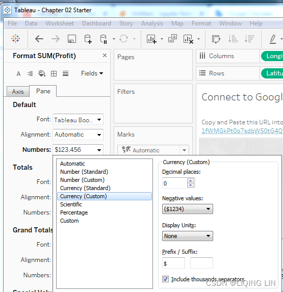
  
  After clicking OK, you should notice that the labels on the map have updated to include currency notation.
• Right-click the Profit field again and select Default properties | Color.... The resulting dialog gives you an option to select and customize the default color encoding of the Profit field. Experiment with various palettes and settings. Notice that every time you click the Apply button, the visualization updates.
  OR
  click drop down menu==>
  
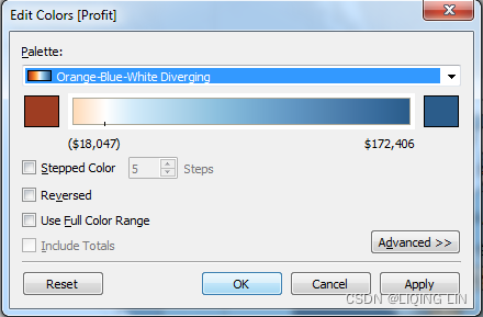
       Diverging palettes (palettes that blend from one color to another) work particularly well for fields such as Profit , which can have negative and positive values. The default center of 0 allows you to fairly easily tell what values are positive or negative based on the color shown.

     Consider using color blind-safe colors in your visualizations. Orange and blue are usually considered one color blind-safe alternative to red and green. Tableau also includes a discrete color-blind safe palette. Additionally, consider adjusting the intensity of the colors考虑调整颜色的强度. 

Shortcuts for connecting to data

     You can make certain connections very quickly. These options will allow you to begin analyzing more quickly:

• Paste data from the clipboard. If you have copied data from a spreadsheet, a table on a webpage, or a text file, you can often paste the data directly into Tableau. This can be done using Ctrl + V, or Data | Paste Data from the menu. The data will be stored as a file and you will be alerted to its location when you save the workbook.
• Select File | Open from the menu. This will allow you to open any data file that Tableau supports, such as text files, Excel files, Access files (not available on macOS), spatial files, statistical files, JSON, and even offline cube ( . cub ) files.
• Drag and drop a file from Windows Explorer or Finder onto the Tableau workspace. Any valid file-based data source can be dropped onto the Tableau workspace, or even the Tableau shortcut on your desktop or taskbar.
• Duplicate an existing connection. You can duplicate an existing Data Source connection by right-clicking and selecting Duplicate. 

Managing data source metadata

     Data sources in Tableau store information about the connection(s). In addition to the connection itself (example, database server name, database, and/or file names), the data source also contains information about all the fields available (such as field name, data type, default format, comments, and aliases). Often, this data about the data is referred to as metadata. 

     Right-clicking a field in the data pane reveals a menu of metadata options. Some of these options will be demonstrated in a later exercise; others will be explained throughout the book. These are some of the options available via right-clicking:

• Renaming the field
• Hiding the field
• Changing aliases for values of dimension (other than date fields)
• Creating calculated fields, groups, sets, bins, or parameters
• Splitting the field
• Changing the default use of a date or numeric field to either discrete or continuous
• Redefining the field as a dimension or a measure
• Changing the data type of the field
• Assigning a geographic role of the field
• Changing defaults for how a field is displayed in a visualization, such as the default colors and shapes, number or date format, sort order (for dimensions), or type of aggregation (for measures)
• Adding a default comment for a field (which will be shown as a tooltip when hovering over a field in the data pane, or shown as part of the description when Describe... is selected from the menu)
• Adding or removing the field from a hierarchy

     Metadata options that relate to the visual display of the field, such as default sort order or default number format, define the overall default for a field. However, you can override the defaults in any individual view by right-clicking the active field on the shelf and selecting the desired options.

Working with extracts instead of live connections 

     Most data sources allow the option of either connecting live or extracting the data. However, some cloud-based data sources require an extract. Conversely, OLAP data sources cannot be extracted and require live connections. 

     When using a live connection, Tableau issues queries directly to the data source (or uses data in the cache, if possible). When you extract the data, Tableau pulls some or all of the data from the original source and stores it in an extract file. Prior to version 10.5, Tableau used a Tableau Data Extract ( .tde ) file. Starting with version 10.5, Tableau uses Hyper extracts ( .hyper ) and will convert .tde files to .hyper as you update older workbooks.

Extracts extend the way in which Tableau works with data. Consider the following diagram: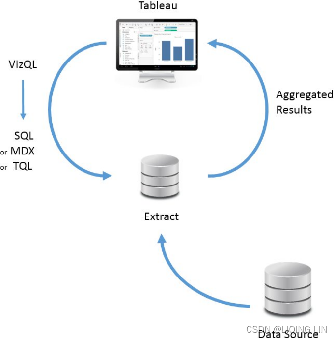 

     The fundamental paradigm of how Tableau works with data does not change, but you'll notice that Tableau is now querying and getting results from the extract. Data can be retrieved from the source again to refresh the extract. Thus, each extract is a snapshot of the data source at the time of the latest refresh. Extracts offer the benefit of being portable and extremely efficient.

Creating extracts

     Extracts can be created in multiple ways, as follows:

• Select Extract on the Data Source screen as follows. The Edit... link will allow you to configure the extract:
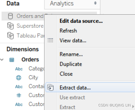
• Select the data source from the Data menu, or right-click the data source on the data pane and select Extract data.... You will be given a chance to set configuration options for the extract, as demonstrated in the following screenshot:
• Developers may create an extract using the Tableau Data Extract API. This API allows you to use Python or C/C++ to programmatically create an extract file. The details of this approach are beyond the scope of this book, but documentation is readily available on Tableau's website.
• Certain tools, such as Alteryx or Tableau Prep, are able to output Tableau extracts.

     When you first create or subsequently configure an extract, you will be prompted to select certain options, as shown here: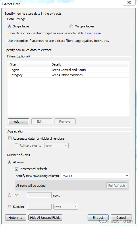
==> Add...  

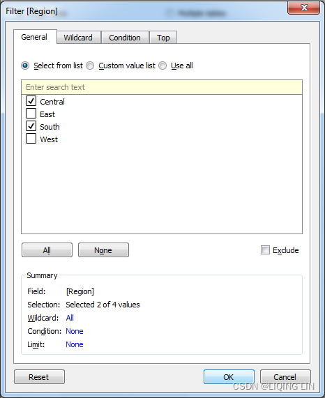
• You may optionally add Extract filters, which limit the extract to a subset of the original source. In this example only, records
  where Region is Central or South==>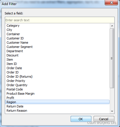
  and where Category is Office Machines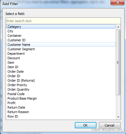==> 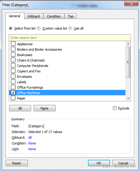will be included in the extract.
• You may aggregate an extract by checking the box. This means that data will be rolled up to the level of visible dimensions and, optionally, to a specified date level, such as year or month.
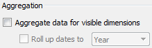
       Visible fields are those that are shown in the data pane. You may hide a field from the Data Source screen or from the data pane by right-clicking a field and selecting Hide. This option will be disabled if the field is used in any view in the workbook. Hidden fields are not available to be used in a view. Hidden fields are not included in an extract as long as they are hidden prior to creating or optimizing the extract.
• In the preceding example, if only the Region and Category dimensions were visible, the resulting extract would only contain two rows of data (one row for Central and another for South). Additionally, any measures would be aggregated at the Region / Category level and would be done with respect to the Extract filters. For example, Sales would be rolled up to the sum of sales in Central/Office Machines and South/Office Machines. All measures are aggregated according to their default aggregation.
• You may adjust the Number of Rows in the extract by including all rows or a sampling of the top N rows in the dataset. If you select all rows, you can indicate an incremental refresh. If your source data incrementally adds records, and you have a field such as an identity column or date field that can be used reliably to identify new records as they are added, then an incremental extract can allow you to add those records to the extract without recreating the entire extract. In the preceding example, any new rows where Row ID is higher than the highest value of the previous extract refresh would be included in the next incremental refresh行 ID 高于上一次数据提取刷新的最大值的任何新行都将包含在下一次增量刷新中.
  
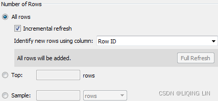
  Incremental refreshes can be a great way to deal with large volumes of data that grow over time. However, use incremental refreshes with care, because the incremental refresh will only add new rows of data based on the field you specify. You won't get changes to existing rows, nor will rows be removed if they were deleted at the source. You will also miss any new rows if the value for the incremental field is less than the maximum value in the existing extract.

Using extracts

     Any data source that is using an extract will have a distinctive icon that indicates the data has been pulled from an original source into an extract, as shown in the following screenshot: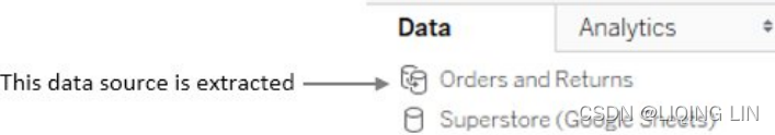 

     The first data connection in the preceding data pane is extracted, while the second is not. After an extract has been created, you may choose to use the extract or not. When you right-click a data source (or Data from the menu and then the data source), you will see the following menu options, as demonstrated in this screenshot:

• 1. Refresh: The Refresh option under the data source simply tells Tableau to refresh the local cache of data.
  • With a live data source, this would requery the underlying data.
  • With an extracted source, the cache is cleared and the extract is requeried, but this Refresh option does not update the extract from the original source. To do that, use Refresh under the Extract sub-menu (see step 4 in this list).
• 2. Extract data...: This creates a new extract from the data source (replacing an existing extract if it exists).
• 3. Use Extract: This option is enabled if there is an extract for a given data source. Unchecking the option will tell Tableau to use a live connection instead of the extract. The extract will not be removed and may be used again by checking this option at any time. If the original data source is not available to this workbook, then Tableau will ask where to find it.
• Extract
  • 4. Refresh: This Refresh option refreshes the extract with data from the original source. It does not optimize the extract for some changes you make (such as hiding fields or creating new calculations).
    • Refresh (Incremental)
      • An incremental refresh will feed in ONLY NEW data in the data set
      • This is usually a lot quicker than a full refresh as it is not querying data already in the extract
      • This will not look at any changes in the original data set, it will only load up NEW rows of data entered into the database
    • Refresh (Full)
      • Full refresh will send a query to the database to return ALL EXISTING ROWS of data from the previous query as well as the new rows
      • This will take longer than an incremental refresh
      • Will look at changes in the underlying data as well (for example if a sales value was to change in your data, the full refresh would pick this up)
  • 5. Append data from file...: This option allows you to append additional files to an existing extract, provided they have the same exact data structure as the original source. This adds rows to your existing extract; it will not add new columns.
  • 6. Optimize(Compute Calculations Now): This will restructure the extract, based on changes you've made since originally creating the extract, to make it as efficient as possible. For example, certain calculated fields may be materialized被具体化 (that is, calculated once so that the resulting value can be stored) and newly hidden columns or deleted calculations will be removed from the extract.
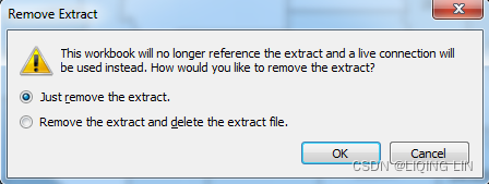
  • 7. Remove: This removes the definition of the extract, optionally deletes the extract file, and resumes a live connection to the original data source.
    
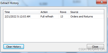
  • 8. History: This allows you to view the history of the extract and refreshes.
    

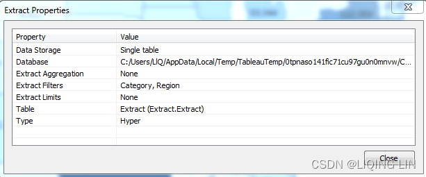
  • 9. Properties: This enables you to view the properties of the extract, such as the location, underlying source, filters, and row limits. 

Performance 

     Prior to 10.5, Tableau Data Extracts ( .tde files) were very efficient columnar databases that performed well with the Tableau data engine. With Tableau 10.5, Tableau introduced the Hyper data engine, which shows remarkable performance gains, especially for large datasets. Both .tde and .hyper extracts will perform faster than most traditional live database connections. This is based on several factors, as follows: 

• Hyper extracts超提取 make use of a hybrid混合 of OLTP(Online transaction processing) and OLAP(Online analytical processing) models, and the engine determines the optimal query. Tableau Data Extracts are columnar列式的 and also very efficient to query.
• Extracts are structured so they can be loaded quickly into memory without additional processing and moved between memory and disk storage, so the size is not limited to the amount of RAM available.
• Many calculated fields are materialized in the extract. The pre-calculated value stored in the extract can often be read faster than executing the calculation every time the query is executed. Hyper extracts extend this by potentially materializing many aggregations. 

     You may choose to use extracts to increase performance over traditional databases. To maximize your performance gain, consider the following actions:

• Prior to creating the extract, hide unused fields. If you have created all desired visualizations, you can click the Hide Unused Fields button on the extract dialog to hide all fields not used in any view or calculation.
• If possible, use a subset of data from the original source. For example, if you have historical data for the last 10 years, but will only need the last two years for analysis, then filter the extract by the Date field.
• Optimize an extract after creating or editing calculated fields, or deleting or hiding fields.
• Store extracts on solid state drives.

Portability and security

     Let's say that your data is hosted on a database server accessible only from inside your office network. Normally, you'd have to be onsite or using a VPN to work with the data. With an extract, you can take the data with you and work offline. 

     An extract file contains data extracted from the source. When you save a workbook, you may save it as a Tableau workbook ( .twb ) file or a Tableau Packaged Workbook ( .twbx ) file. A workbook ( .twb ) contains definitions for all the connections, fields, visualizations, and dashboards, but does not contain any data or external files, such as images. When you save a packaged workbook ( .twbx ), any extracts and external files are packaged together in a single file with the workbook.

     A packaged workbook using extracts can be opened with Tableau Desktop, Tableau Reader, and published to Tableau Public or Tableau Online.

     A packaged workbook file ( .twbx ) is really just a compressed .zip file. If you rename the extension from .twbx to .zip , you can access the contents as you would any other .zip file. You may also consider associating the .twbx extension with your ZIP utility so you won't have to rename the files. 

     There are a couple of security considerations to keep in mind when using an extract: 

• The extract is made using a single set of credentials. Any security layers that limit which data can be accessed according to the credentials used will not be effective after the extract is created. An extract does not require a username or password. All data in an extract can be read by anyone.
• Any data for visible (non-hidden) fields contained in an extract file ( .hyper or .tde ), or an extract contained in a packaged workbook ( .twbx ), can be accessed even if the data is not shown in the visualization. Be very careful to limit access to extracts or packaged workbooks containing sensitive or proprietary[prəˈpraɪəteri]专有的,私有的,私密的 data. 

     The story is told of an employee who sent a packaged workbook containing HR data to others in the company. Even though none of the dashboards displayed sensitive data, the extract contained it. It wasn't long before everyone in the company knew everyone else's salary and the original individual was no longer an employee.

When to use an extract

     You should consider various factors when determining whether or not to use an extract. In some cases, you won't have an option (for example, OLAP requires a live connection and some cloud-based data sources require an extract). In other cases, you'll want to evaluate your options. 

In general, use an extract when:

• You need better performance than you can get with the live connection.
• You need the data to be portable.
• You need to use functions that are not supported by the database data engine (for example, MEDIAN is not supported with a live connection to SQL Server).
• You want to share a packaged workbook. This is especially true if you want to share a packaged workbook with someone who uses the free Tableau Reader, which can only read packaged workbooks with data extracted.

In general, do not use an extract when you have any of the following use cases:

• You have sensitive data that should not be accessible by certain users, or you have no control over无法控制 who will be able to access the extract. However, you may hide sensitive fields prior to creating the extract, in which case they are no longer part of the extract.
• You need to manage security based on login credentials. (However, if you are using Tableau Server, you may still use extracted connections hosted on Tableau Server that are secured by login. We'll consider sharing your work with Tableau Server in Chapter 12 , Sharing Your Data Story).
• You need to see changes in the source data updated in real time.
• The volume of data makes the time required to build the extract impractical. The number of records that can be extracted in a reasonable amount of time will depend on factors such as the data types of fields, the number of fields, the speed of the data source, and network bandwidth. The hyper engine typically builds the new .hyper extracts much faster than the older .tde files were built.

Tableau file types

     In addition to the file types mentioned previously, there are quite a few other file types associated with Tableau. The following are some of the Tableau file types:

• Workbooks (.twb) – Tableau workbook files have the .twb file extension. Workbooks hold one or more worksheets, plus zero or more dashboards and stories.
  
  它包含在每个视图中使用的字段的详细信息以及应用于度量的聚合公式。还应用了格式和样式。它还包含数据源连接信息和为该连接创建的任何元数据信息。
  
  ( .twb ): A Tableau Workbook—an XML file containing definitions for all sheets, data sources, preferences, and formatting. It does not contain any data.
• Packaged Workbooks (.twbx) – Tableau packaged workbooks have the .twbx file extension. A packaged workbook is a single zip file that contains
  • a workbook(.twb) along with
  • any supporting local file data (OR any data extracts ( .tde )) and
  • background images (OR any other external files (such as images, or text/Excel files for data sources that are not extracted)).
  • This format is the best way to package your work for sharing with others who don’t have access to the original data.(前提是它不需要来自服务器的数据) For more information, see Packaged Workbooks - Tableau.
• Data Source (.tds) – Tableau data source files have the .tds file extension. Data source files are shortcuts for quickly connecting to the original data that you use often. Data source files do not contain the actual data but rather
  • the information necessary to connect to the actual data as well as
    在连接细节中，它存储源类型（excel/relational/sap等）以及列的数据类型
  • any modifications you've made on top of the actual data such as
    • changing default properties,
    • creating calculated fields,
    • adding groups, and so on.
    • For more information, see Save Data Sources - Tableau.
  • (.tds) :  Tableau Data Source file—an XML file containing the definition of a data source (the server name, file path, and so on), but does not contain the data. You can export a data source as a .tds file by right-clicking the data source and selecting Add to Saved Data Sources. Any .tds files in your My Tableau Repository Data Sources(C:\Users\LlQ\Documents\My Tableau Repository) directory will show as data connection shortcuts on the Home Screen.
• Packaged Data Source (.tdsx) – Tableau packaged data source files have the .tdsx file extension. A packaged data source is a zip file that contains
  • the definition of the data source file (.tds) described above as well as
  • any local file data such as
    • extract files (.hyper or .tde),
    • text files,
    • Excel files,
    • Access files, and
    • local cube files本地多维数据集文件.
  • Use this format to create a single file that you can then share with others who may not have access to the original data stored locally on your computer. For more information, see Save Data Sources - Tableau.
  • You may create packaged data sources in the same way you create .tds files, selecting .tdsx as the file type.
• Extract (.hyper or .tde) – Depending on the version the extract was created in,(此文件包含高压缩的柱状数据格式的.twb文件中使用的数据。这有助于存储优化。它还保存在分析中应用的聚合计算。此文件应刷新以从源获取更新的数据)
  Tableau extract files can have either the .hyper(A Hyper extract—a binary file containing data extracted from another source. This is the extract format used by Tableau 10.5 and later, which utilizes the much faster and scalable hyper engine)
  or .tde(A Tableau Data Extract—a binary file containing data extracted from another source. The .tde file by itself does not contain information about the original data source.) file extension. Extract files are
  • a local copy of a subset
  • or entire data set that you can use to share data with others, when you need to work offline, and improve performance.
  • For more information, see Extract Your Data - Tableau.
• Bookmarks (.tbm) – Tableau bookmark files have the .tbm file extension. Bookmarks contain a single worksheet and are an easy way to quickly share your work. For more information, see Save Your Work - Tableau.
  • A Tableau Bookmark file—an XML file containing a definition of a static snapshot of a single view and associated data sources. As sheets can now be copied and pasted from one workbook to another, this file type is largely not needed. You can create bookmarks and import them into other workbooks from the Window menu.
• Tableau偏好设置.tps - 此文件存储所有工作簿中使用的颜色首选项。它主要用于在用户之间保持一致的外观和感觉
  • Tableau Preferences—an XML file containing preference defaults for Tableau Desktop, including UI elements and color palettes.
• .tfl : A Tableau Flow file—a file defining a Tableau Prep flow. Tableau Desktop does not read this file type.
• .tflx : A Packaged Tableau Flow file—a compressed .zip file containing the .tfl file and extracts of the file-based data sources for the flow. Tableau Desktop does not read this file type.
• .tld/.tlf/.tlq/.tlr : A Tableau License file— Disconnected / File / Request / Return / Response file types are used in license activation.
• .tms : A Tableau Map Source file—an XML file type used to specify map services and configuration available to Tableau.
• .tmsd : A Tableau Map Source Defaults file—an XML file containing defaults for map services
• .tsvc : The Tableau Atom Service file type.

Joins and blends

     Joining tables and blending data sources are two different ways to link related data together in Tableau. Joins are performed to link tables of data together on a row-by-row basis. Blends are performed to link together multiple data sources at an aggregate level.

Joining tables

     Most databases have multiple tables of data that are related in some way. Additionally, with Tableau 10 and later, you are able to join together tables of data across various data connections for many different data sources. As we'll see, Tableau makes it very easy to join together tables of data relatively easy.

Consider, for example, tables such as these:

     The primary table is the Hospital Visit table, which has a record for every visit of a patient to the hospital and includes details such as admission type (examples include inpatient住院病人, outpatient门诊, and ER急诊室). It also contains key fields that link a visit to a Primary Physician, Patient, and Discharge Details.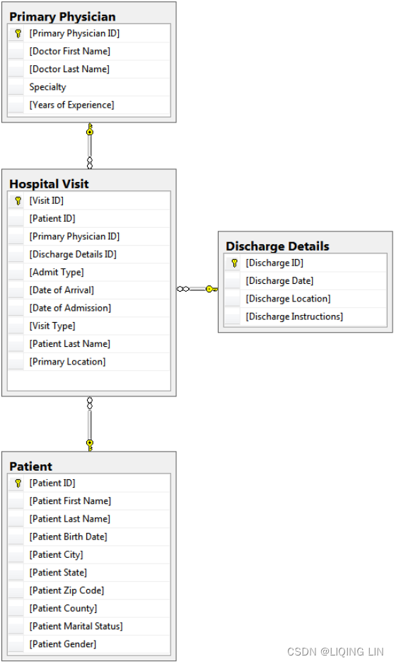

     When you connect to the database in Tableau, you'll see the tables listed on the left and will have the option to drag and drop them into the data source designer.

     Typically, you'll want to start by dragging the primary table into the designer. In this case, Hospital Visit contains keys for joining additional tables. Those tables should be dragged and dropped after the primary table.

     If key fields and relationships have been defined in the database, Tableau will automatically create the joins as you add additional tables. Otherwise, it will attempt to match field names. In any case, you may adjust the joins as needed. The preceding tables will look similar to the following diagram when dropped into the designer: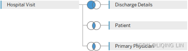

     You may adjust the join by clicking the small diagram between the tables. The diagram indicates what kind of join is used. For example, the join between Hospital Visit and Patient is an Inner Join because it is assumed that every visit will have a patient and every patient will have a visit. However, the join between Hospital Visit and Discharge Details is a left join because some records in Hospital Visit may be for patients still in the hospital (so they haven't been discharged还没有出院).

     Clicking on the diagram will allow you to select a different type of join and define which fields are part of the join.

You may specify the following types of joins:

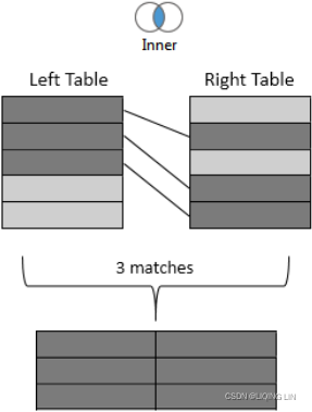
• Inner: Only records that match the join condition from both the table on the left and the table on the right will be kept. In the following example, only the three matching rows are kept in the results:
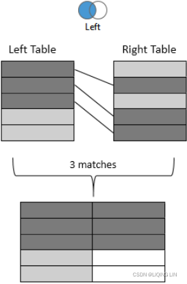
• Left: All records from the table on the left will be kept. Matching records from the table on the right will have values in the resulting table, while unmatched records will contain NULL values for all fields from the table on the right. In the following example, the five rows from the left table are kept with NULL results for right values that were not matched:
• Right: All records from the table on the right will kept. Matching records from the table on the left will result in values, while unmatched records will contain NULL values for all fields from the table on the left. Not every data source supports a right join. If it is not supported, the option will be disabled. In the following example, the five rows from the right table are kept with NULL results for left values that were not matched:
• Full Outer: All records from tables on both sides will be kept. Matching records will have values from the left and the right. Unmatched records will have NULL values where either the left or the right matching record was not found. Not every data source supports a full outer join. If it is not supported, the option will be disabled. In the following example, all rows are kept from both sides with NULL values where matches were not found:

Cross database joins

     With Tableau, you have the ability to join (at a row level) across multiple different data connections. Joining across different data connections is referred to as a cross database join. For example, you can

• join SQL Server tables with text files or Excel files, or
• tables in one database with tables in another, even if those are on a different server.

This opens up all kinds of possibilities for supplementing your data or analyzing data from disparate sources. 

     Consider the hospital data mentioned previously. It would not be uncommon for billing data to be in a separate system from patient care data. Let's say you had a file for patient billing that contained data you wanted to include in your analysis of hospital visits. You would be able to accomplish this by adding the text file as a data connection and then joining it to the existing tables, as follows: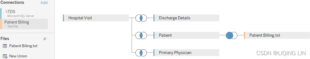
     You'll notice that the interface on the Data Source screen includes an Add link that allows you to add data connections to a data source. Clicking on each connection will allow you to drag and drop tables from that connection into the Data Source designer and specify the joins as you desire. Each data connection will be color-coded so that you can immediately identify the source of various tables in the designer.

     In the preceding example, the Patient Billing.txt text file has been joined to the Patient table from SQL Server. 

     With all joins, including cross-data connection joins, you will need to make certain that you have field(s) that are shared in common between the tables. For example, to join Patient Billing.txt to the Patient table, there will need to be some kind of patient ID or account number that can be matched. Cross database joins also require that the data types be identical. You can use a join calculation to change the type if needed.

Blending data sources

     Data blending is a powerful and innovative feature in Tableau. It allows you to use data from multiple data sources in the same view. Often these sources may be different types. For example, you can blend data from Oracle with data from Excel. You can blend Google Analytics data with a spatial file. Data blending also allows you to compare data at different levels of detail. Some advanced uses of data blending will be covered in Chapter 8 , Digging Deeper: Trends, Clustering, Distributions and Forecasting. For now, let's consider the basics and a simple example. 

     Data blending is done at an aggregate level and involves different queries sent to each data source, unlike joining, which is done at a row level and involves a single query to a single data source. A simple data blending process involves several steps, as shown in the following diagram: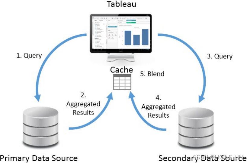

We can see the following from the preceding diagram:

• 1. Tableau issues a query to the primary data source.
• 2. The underlying data engine returns aggregate results.
• Step 3. Tableau issues another query to the secondary data source. This query is filtered based on the set of values returned from the primary data source for dimensions that link the two data sources.
• Step 4. The underlying data engine returns aggregate results from the secondary data source.
• 5. The aggregated results from the primary data source and the aggregated results from the secondary data source are blended together in the cache. 

     It is important to note how data blending is different from joining. Joins are accomplished in a single query and results are matched row-by-row. Data blending occurs by issuing two separate queries and then blending together the aggregate results.

     There can only be one primary source, but there can be as many secondary sources as you desire. Steps 3 and 4 will be repeated for each secondary source. When all aggregate results have been returned, Tableau will match the aggregate rows based on linking fields.

     When you have more than one data source in a Tableau workbook, whichever source you use first in a view becomes the primary source for that view.

     Blending is view-specific. You can have one data source as the primary in one view and the same data source as the secondary in another. Any data source can be used in a blend, but OLAP cubes, such as SSAS, must be used as the primary source.

     Linking fields are dimensions which are used to match data blended between primary and secondary data sources. Linking fields define the level of detail for the secondary source. Linking fields are automatically assigned if fields match by name and type between data sources. Otherwise, you can manually assign relationships between fields by selecting, from the menu, Data | Edit Relationships, as follows: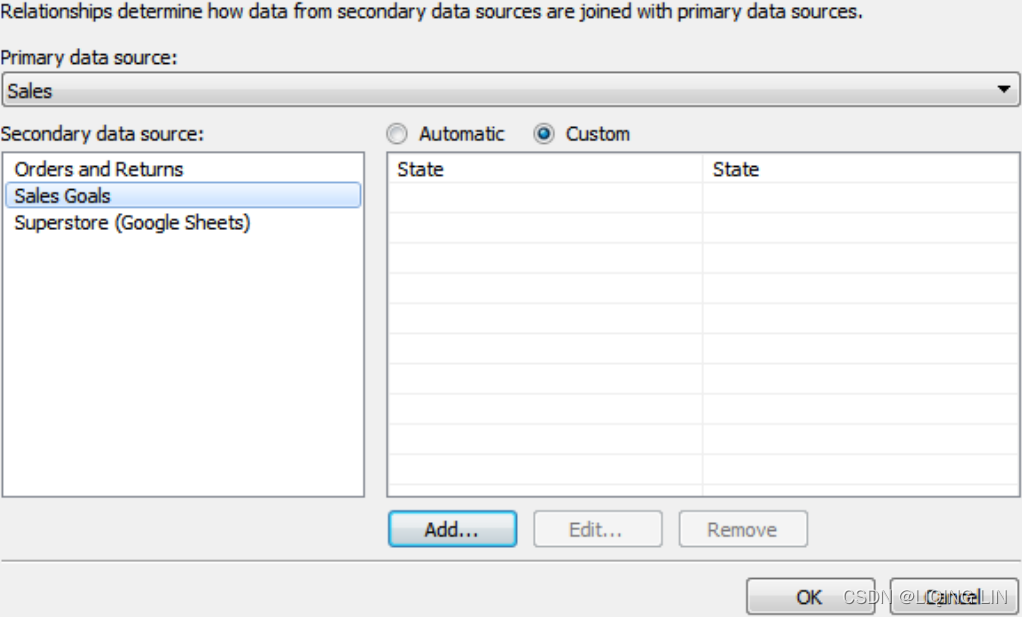

     The Relationships window will display the relationships recognized between different data sources. You can switch from Automatic to Custom to define your own linking fields.

     Linking fields can be activated or deactivated for blending in a view. Linking fields used in the view will usually be active by default, while other fields will not. You can, however, change whether a linking field is active or not by clicking the link icon next to a linking field in the Data pane.

     Additionally, use the Edit Data Relationships screen to define the fields that will be used for cross-data source filters, which are discussed in the next section (Filtering).

A blending example

     The following screenshot shows a simple example of data blending in action: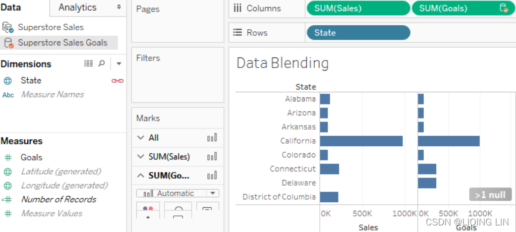

     There are two data source connections defined in this workbook, one for the Superstore data and the other for Superstore Sales Goals . The Superstore data source is the primary data source in this view (indicated by the blue checkmark) and Superstore Sales Goals is the secondary source (indicated by the orange checkmark). Active fields in the view that are from the secondary data source are also indicated with an orange checkmark icon.

     The Sales measure has been used from the primary source and the Goals from the secondary sources. In both cases, the value is aggregated. The State dimension is an active linking field, indicated by the orange chain link icon next to the field in the data pane. Both measures are being aggregated at the level of State (sales by state in Superstore Sales, and goals by state in Superstore Sales Goals ) and then matched by Tableau based on the value of the linking field State .

     Data blending will be done based on an exact match of the dimension values for the linking field(s). Be careful, as this can lead to some matches being missed. You'll notice the indicator in the lower-right of the preceding screenshot, which indicates > 1 null (at least one null value).

     An examination of the data reveals that the State value in Superstore Sales is District of Columbia, while it is DC in the Superstore Sales Goals data source. You'll either need to fix the values in the data source, create a calculated field to change values, or change the alias of the value in one data source to match the value in another. For example, you could right-click District of Columbia in the row header, select Edit alias... and set the value to DC.

     We'll see some examples of editing aliases throughout the book. Take note of the following definition:

     An alias is an alternate value for a dimension value that will be used for display and data blending. Aliases for dimensions can be changed by right-clicking row headers or using the menu on the field in the view or in the Data Pane, and selecting the option for editing aliases.

Filtering data

     Often, you will want to filter data in Tableau in order to perform an analysis on a subset of data, narrow your focus缩小关注范围, or drill into detail深入了解细节. Tableau offers multiple ways to filter data.

     If you want to limit the scope of your analysis to a subset of data, you can filter the data at the source using one of the following techniques:

• Data Source Filters are applied before all other filters and are useful when you want to limit your analysis to a subset of data. These filters are applied before any other filters.
• Extract Filters limit the data that is stored in an extract ( .tde or .hyper ). Data source filters are often converted into extract filters if they are present when you extract the data.
• Custom SQL Filters can be accomplished using a live connection with custom SQL, which has a Tableau parameter in the WHERE clause. 

Additionally, you can apply filters to one or more views using one of the following techniques:

• Drag and drop fields from the data pane to the Filters shelf.
• Select one or more marks or headers in a view and then select Keep Only or Exclude, as shown here:.
• Right-click any field in the data pane or in the view, and select Show Filter. The filter will be shown as a control (examples include a drop-down list and checkbox) to allow the end user of the view or dashboard the ability to change the filter.
•  Use an action filter. We'll look more at filters and action filters in the context of dashboards

     Each of these options adds one or more fields to the Filters shelf of a view. When you drop a field on the Filters shelf, you will be prompted with options to define the filter. The filter options will differ most noticeably based on whether the field is discrete or continuous. Whether a field is filtered as a dimension or as a measure will greatly impact how the filter is applied and the results. 

Filtering discrete (blue) fields

     When you filter using a discrete field, you will be given options for selecting individual values to keep or exclude. For example, when you drop the discrete Department dimension onto the Filters shelf, Tableau will give you the following options: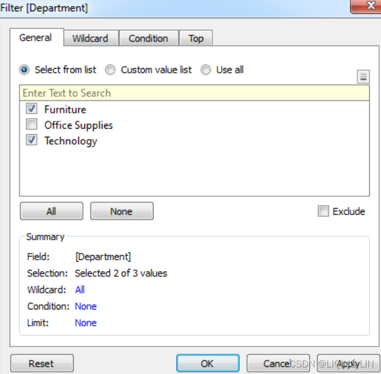

     The Filter options include General, Wildcard, Condition, and Top tabs. Your Filter can include options from each tab. The Summary section on the General tab will show all options selected:

• The General tab allows you to select items from a list (you can use the custom list add items manually if the dimension contains a large number of values that takes a long time to load.) You may use the Exclude option to exclude the selected items.
• The Wildcard tab allows you to match string values that contain, start with, end with, or exactly match a given value.
• The Condition tab allows you to specify conditions based on aggregations of other fields that meet conditions (for example, a condition to keep any Department where the sum of sales was greater than $1,000,000). Additionally, you can write a custom calculation to form complex conditions.
• The Top tab allows you to limit the filter to only the top or bottom items. For example, you might decide to keep only the top five items by the sum of sales.

     Discrete measures (except for calculated fields using table calculations) cannot be added to the Filters shelf. If the field holds a date or numeric value, you can convert it to a continuous field(e.g. {classes: 1,2,3,...}) before filtering. Other data types will require the creation of a calculated field to convert values you wish to filter into continuous numeric values. 

Filtering continuous (green) fields

     If you drop a continuous dimension onto the Filters shelf, you'll get a different set of options. Often, you will first be prompted as to how you want to filter the field, as follows: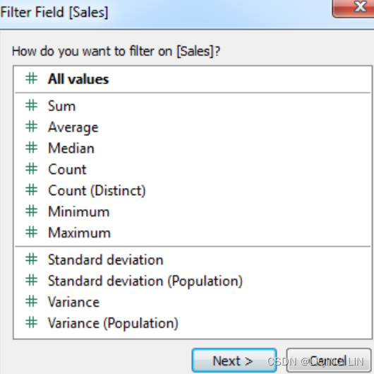

The options here are divided into two major categories:

• All Values: The filter will be based on each individual value of the field. For example, an All Values filter keeping only sales above $100 will evaluate each record of underlying data and keep only individual sales above $100.
• Aggregation: The filter will be based on the aggregation specified (for example, Sum, Average, Minimum, Maximum, Standard deviation, and Variance) and the aggregation will be performed at the level of detail of the view. For example, a filter keeping only the sum of sales above $100,000 on a view at the level of category will keep only categories that had at least $100,000 in total sales.

     Once you've made a selection (or if the selection wasn't applicable for the field selected), you will be given another interface for setting the actual filter, as follows: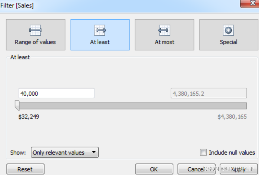

     Here, you'll see options for filtering continuous values based on a range with a start, end, or both. The Special tab gives options for showing all values, NULL values, or non-NULL values.

Filtering dates

     We'll take a look at the special way Tableau handles dates in the Visualizing Dates and Times section of Chapter 3 , Venturing on to Advanced Visualizations. For now, consider the options available when you drop an Order Date field onto the Filters shelf, as follows:

The options here include the following:

• Relative date: This option allows you to filter a date based on a specific date (for example, keeping the last three weeks from today, or the last six months from January 1).
• Range of dates: This option allows you to filter a date based on a range with a starting date, ending date, or both.
• Date Part: This option allows you to filter based on discrete parts of dates, such as Years, Months, Days or combinations of parts, such as Month/Year.
• Individual dates: This option allows you to filter based on each individual value of the date field in the data.
• Count or Count (Distinct): This option allows you to filter based on the count, or distinct count, of date values in the data.

Other filtering options

You will also want to be aware of the following options when it comes to filtering:

• You may display a filter control for nearly any field by right-clicking it and selecting Show Filter. The type of control depends on the type of field, whether it is discrete or continuous, and may be customized by using the little drop-down arrow at the upper-right of the filter control.
• Filters may be added to the Context. Any filters added to the context are evaluated first and result in what can be thought of as a subset of the data. Other filters and calculations (such as computed sets and fixed level of detail calculations) are based on the subset of data. This can be useful if, for example, you want to filter to the top five customers, but want to be able to first filter to a specific region. Making Region a context filter ensures that the top five filter is calculated in the context of the Region filter.
• Filters may be set to show all values in the database, all values in the context, all values in a hierarchy, or only values that are relevant based on other filters. These options are available via the drop-down menu on the Filter control.
• By default, any field placed on the Filters shelf defines a filter that is specific to the current view. However, you may specify the scope by using the menu for the field on Filters shelf. Select Apply to and choose one of the following options:
  • All related data sources: All data sources will be filtered by the value(s) specified. The relationships of fields are the same as blending (that is, the default by name and type match, or customized through the Data | Edit Relationships... menu option). All views using any of the related data sources will be affected by the filter. This option is sometimes referred to as cross-data source filtering.
  • Current Data Source: The data source for that field will be filtered. Any views using that data source will be affected by the filter.
  • Selected Worksheets: Any worksheets selected that use the data source of the field will be affected by the filter.
  • Current Worksheet: Only the current view will be affected by the filter.
• When using Tableau Server, you may define user filters that allow you to provide row-level security by filtering based on user credentials.

Summary

     This chapter covered key concepts of how Tableau works with data. Although you will not usually be concerned with what queries Tableau generates to query underlying data engines, having a solid understanding of Tableau's paradigm范例 will greatly aid you as you analyze data.

     We looked at multiple examples of different connections to different data sources, considered the benefits and potential drawbacks of using data extracts, considered how to manage metadata, dove into details on joins and blends, and finally, took a look at options for filtering data.

     Working with data is fundamental to everything you do in Tableau. Having an understanding of connecting to various data sources, working with extracts, customizing metadata, and the difference between joins and blends, will be key as you begin deeper analysis and more complex visualizations, such as those covered in the next chapter.