学习MATLAB数值微积分

绪论

Today:
•Polynomial differentiation and integration 多项式的微分和积分
•Numerical differentiation and integration 数值的微分和积分

Polynomial Differentiation 多项式微分

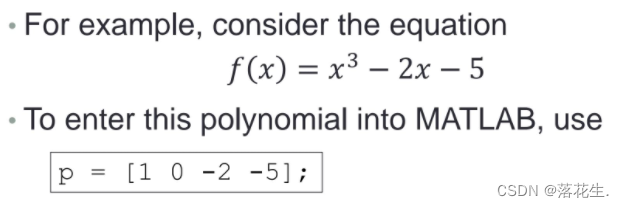
Representing Polynomials in MATLAB

•Polynomials were represented as row vectors
多项式可以用行向量来表示

Values of Polynomials:polyval() 多项式取值

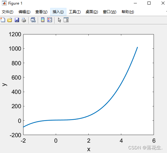
a=[9,-5,3,7];x=-2:0.01:5;
f=polyval(a,x);
plot(x,f,'LineWidth',2);
xlabel('x');
ylabel('y');
set(gca,'FontSize',14)

运行结果

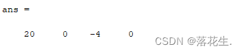
Polynomial Differentiation:polyder() 多项式微分

p=[5 0 -2 0 1];
polyder(p)

结果

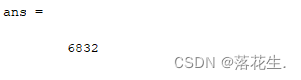
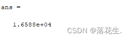
求微分后在x=7处的导数值
加上代码

polyval(polyder(p),7)

结果

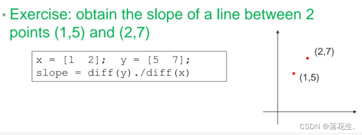
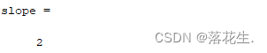
Exercise

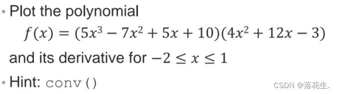
代码

x=-2:0.005:1;       %此处步长对短线的密集程度没有表现出影响
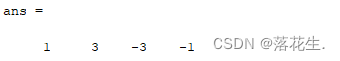
p1=[5 -7 5 10];p2=[4 12 -3];
p=conv(p1,p2);
f=polyval(p,x);
polyder(p);
g=polyval(polyder(p),x);
hold on
plot(x,f,"LineStyle","--","Color",[0,0,1],"LineWidth",2);
plot(x,g,'-r','LineWidth',2)
xlabel('x');
legend('f(x)',"f'(x)");   %注意f’（x）的编辑方式

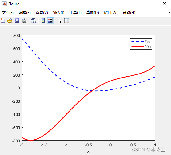
结果

代码解释
conv
卷积和多项式乘法
w = conv(u,v) 返回向量 u 和 v 的卷积。如果 u 和 v 是多项式系数的向量，对其卷积与将这两个多项式相乘等效。
w = conv(u,v,shape) 返回如 shape 指定的卷积的分段。例如，conv(u,v,‘same’) 仅返回与 u 等大小的卷积的中心部分，而 conv(u,v,‘valid’) 仅返回计算的没有补零边缘的卷积部分。

Polynomial Integration 多项式积分

polyint() 积分

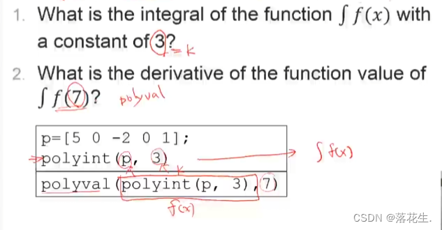
前两行执行的结果依然是多项式
polyint(p,3)中的“3”表示积分以后在后面加的常数为3.
结果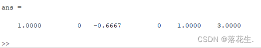
积分后取得的多项式在x=7处的取值
结果

Numerical Differentiation 数值微分

Differences:diff() 差分

•diff()
calculates the differences between adjacent elements of a vector
差分和近似导数
Y = diff(X) 计算沿大小不等于 1 的第一个数组维度的 X 相邻元素之间的差分：

x=[1 2 5 2 1];
diff(x)

输出

练习

结果

运行下图代码

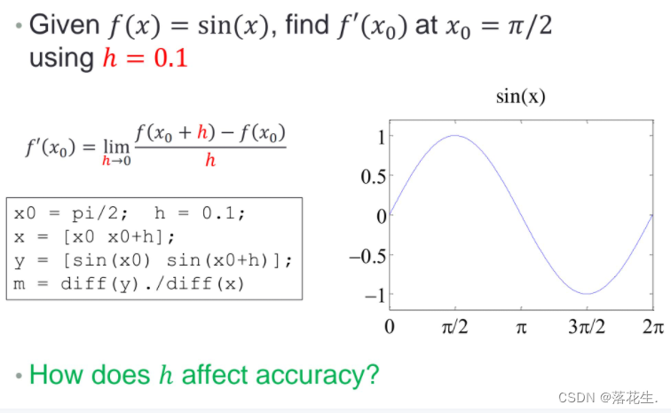
调整h的值去观察误差（sinx在x=0处的导数为0）

h	Error of f’(x0)
0.1	-0.0500
0.01	-0.0050
0.001	-5.0000e-04
0.0001	5.0000e-05
0.00001	-5.0000e-06
0.000001	-5.0004e-07
0.0000001	-4.9960e-08

How to Find the f′ over An Interval[0,2pi]?

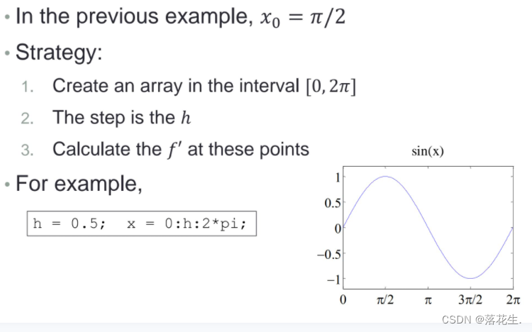
代码

h=0.5;
x=0:h:2*pi;
y=sin(x);
m=diff(y)./diff(x);
plot(x,y,0:h:2*pi-h,m,'Marker','o');
set(gca,"YLim",[-1.2,2]);
set(gca,'XTICK',0:pi/2:2*pi,'FontSize',20)
set(gca,'XTickLabel',{'0','\pi/2','\pi','3\pi/2','2\pi'});
legend('sin(x)',"sin'(x)");

运行结果

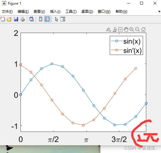
这个2pi并没有出现。

Various Step Size 变化的步长

• The derivatives of f(x)=sin(x) calculated using various ℎ values

g = colormap(lines);
hold on;
for i=1:4
x = 0:power(10, -i):pi;
y = sin(x);
m = diff(y)./diff(x);
plot(x(1:end-1),m, 'Color', g(i,:));
end
hold off;
set(gca,'XLim', [0, pi/2]);
set(gca,'YLim', [0, 1.2]);
set(gca,'FontSize', 18);
set(gca,'FontName','Latex');
set(gca,'XTick', 0:pi/4:pi/2);
set(gca,'XTickLabel', {'0','\pi/4', '\pi/2'});
h = legend('h=0.1','h=0.01','h=0.001','h=0.0001');
set(h,'FontName','Times New Roman');
box on;

运行结果

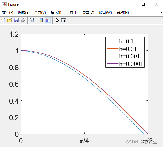
1. C = power(A,B) 是执行 A.^B 的替代方法，但很少使用。它可以启用类的运算符重载。
2. x(1:end-1)就是去掉x中的最后一个值，保证画图时两个变量数目一致
3. color用的颜色是g（i,:）应该是从lines中挑选4个颜色赋予4条曲线。

Exercise

•Given f(x)=e^-xsin(x²/2),plot the approximate derivatives f′ of ℎ=0.1,0.01,and 0.001
代码

g=colormap("lines");
hold on
for i=1:3
    x=0:power(10,-i):2*pi;
    f=exp(-x).*sin(x.^2/2);
    m=diff(f)./diff(x);
    plot(x(1:end-1),m,"Color",g(i,:));
end
hold off
set(gca,'XLim',[0,2*pi]);
set(gca,"YLim",[-0.25,0.25]);
set(gca,'Fontsize',18);
set(gca,'FontName','Latex');
set(gca,'XTick',0:pi/2:2*pi);
set(gca,'XTickLabel',{'0','\pi/2','\pi','3\pi/2','2\pi'});
h=legend('h=0.1','h=0.01','h=0.001');
set(h,"FontName",'Times New Roman');
box on

运行结果

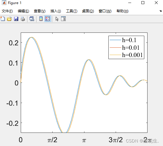
写代码运行时存在的一个问题

正确应该是
f=exp(-x).*sin(x.^2/2);

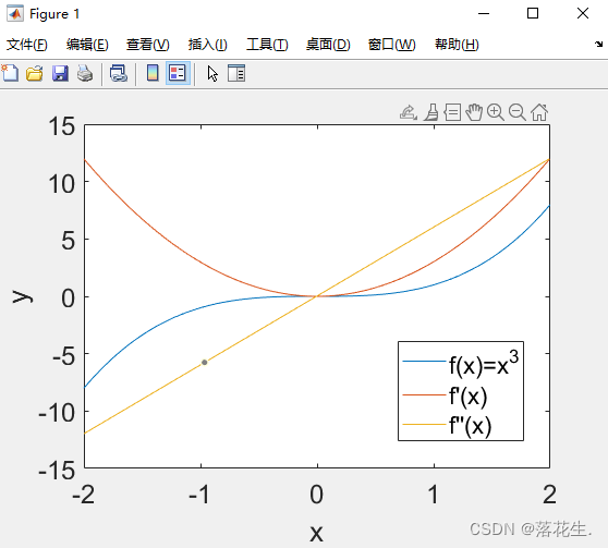
Second and Third Derivatives 二阶三阶微分

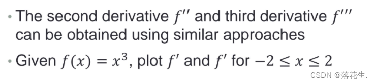
代码

x=-2:0.005:2;
y=x.^3;
m=diff(y)./diff(x);
m2=diff(m)./diff(x(1:end-1));
plot(x,y,x(1:end-1),m,x(1:end-2),m2);
xlabel('x','FontSize',18);
ylabel('y','FontSize',18)
legend('f(x)=x^3',"f'(x)","f''(x)");
set(gca,'FontSize',18);

运行结果

Numerical Integration 数值积分

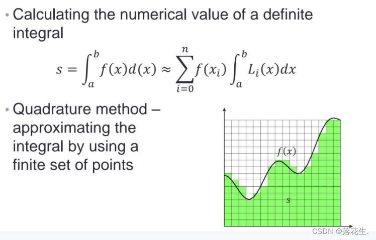
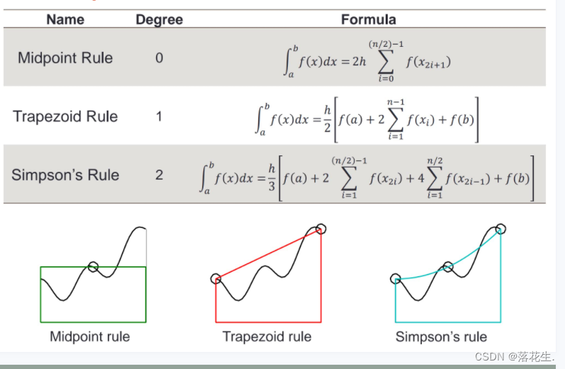
Numerical Quadrature Rules

一共有两种方法：1：取中间值。2：取梯形

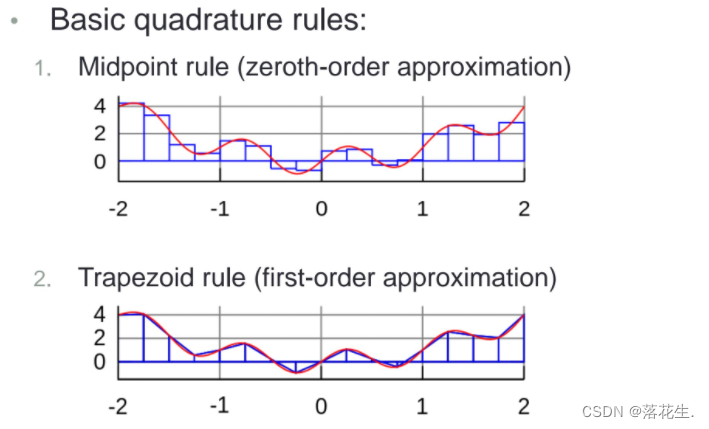
Midpoint Rule 中间值法

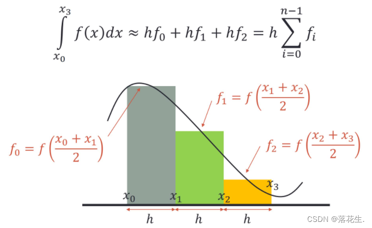
例子

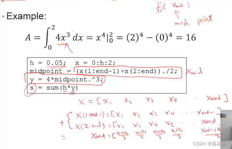
代码

h=0.05;
x=0:h:2;
midpoint=(x(1:end-1)+x(2:end))./2;    %求中点
y=4*midpoint.^3;    %中点对应的y值
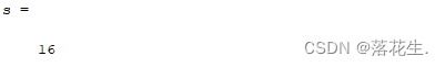
s=sum(h*y)          %乘积求和

运行结果

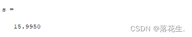
可以看出结果已经很接近答案，精度已经很高，如果想进一步提高精度可以尝试将步长h变得更短。

Trapezoid Rule 梯形法

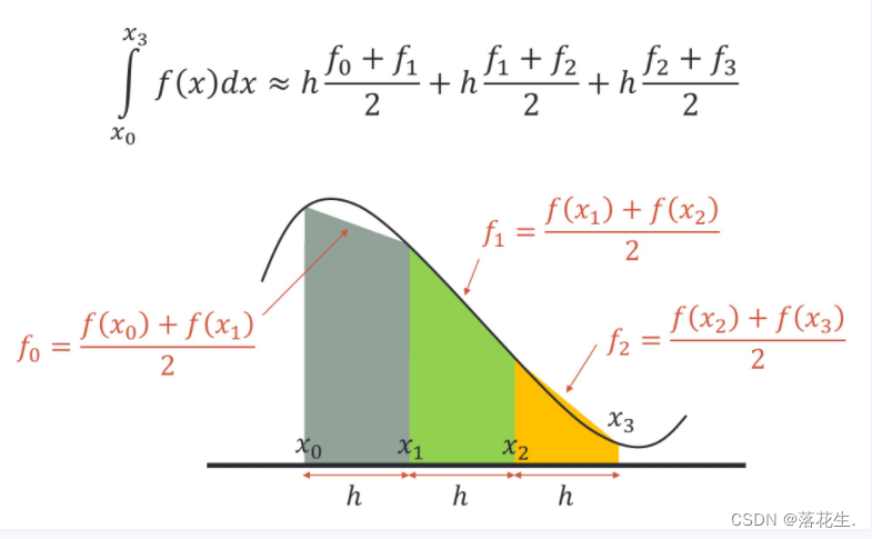
使用到的语法：trapz()

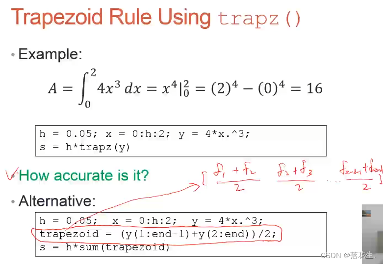
第一段代码运行结果

第二段代码运行结果

再介绍一种更加精准的积分方法

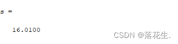
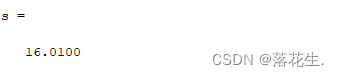
Second-order Rule:1/3Simpson’s 辛普森规则

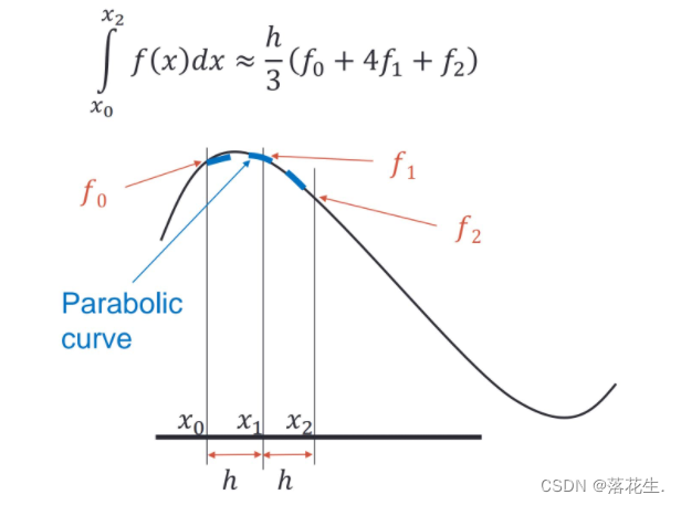
例子

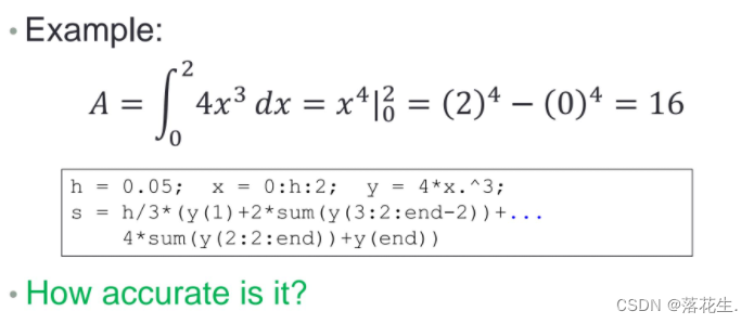
代码

h=0.05;
x=0:h:2;
y=4*x.^3;
s=h/3*(y(1)+2*sum(y(3:2:end-2))+4*sum(y(2:2:end))+y(end))

运行结果

显然，此时的运行结果是比较精确的

下面来对比一下三种积分方式

Comparison 积分方式对比

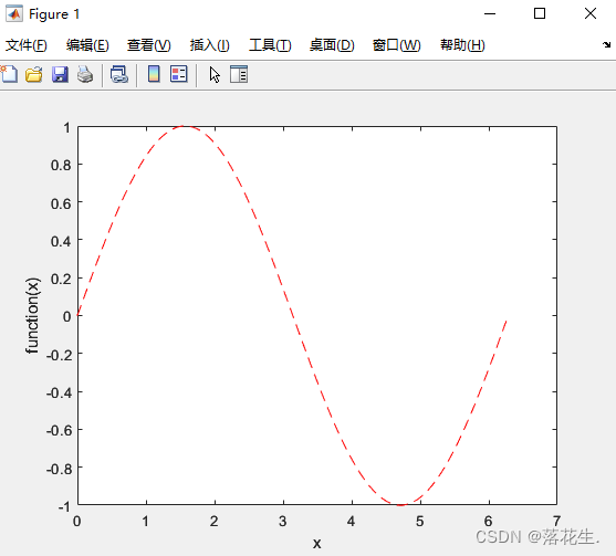
Review of Function Handles (@)

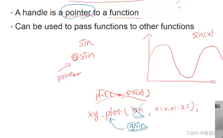
例子

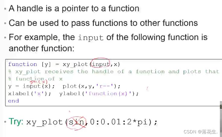
此时输入sin,是无法运行的。需要放置@sin才能运行。@sin是这个function的point。
需要把代码保存放在文件夹内，才能在命令行窗口引用，
在命令行窗口输入

xy_plot(@sin,0:0.01:2*pi)

运行结果

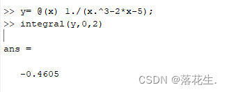
Numerical Integration:integral()

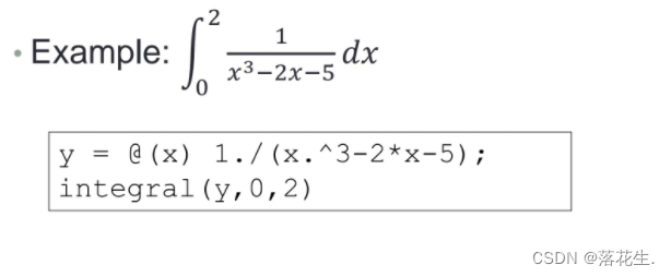
在命令行窗口中执行得到

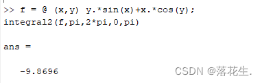
Double and Triple Integrals 二重三重积分

在编辑器的文件里输入代码

f = @ (x,y) y.*sin(x)+x.*cos(y);
integral2(f,pi,2*pi,0,pi)

得到

在上面新建的xy_plot.m中输入上述代码得到

而直接在命令行窗口输入代码得到结果

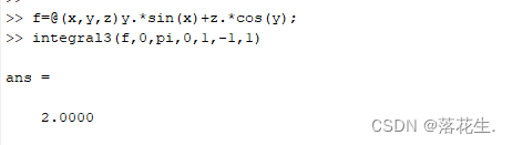
举一个三重积分的例子

在命令行窗口输入指令得到

最后这种方法比较简单好用，可以作为前几种方法的补充。