MATLAB FFT变换中，数字频率与模拟频率的转换关系

我们通常所说的模拟频率，是以Hz为单位的。常用 f 表示。其含义对应于点单位圆上上每秒钟转过的圈数。在模拟世界中，我们也通常用Ω来代表模拟角频率，单位为rad/s。其含义对应于点单位圆上上每秒钟转过的角度。
Ω与f的相互转化关系为： Ω = 2*pi*f。
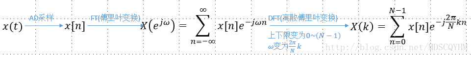
数字频率ω与模拟角频率 Ω和采样频率Fs密切相关。在数字信号处理中，实际是以一定的时间间隔T（T=1/Fs）采样模拟信号得到数字信号的。
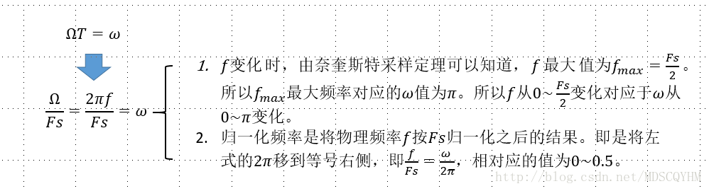
假设模拟信号为 sin( Ωt+θ)，则以采样频率Fs采样该信号得到：sin( ΩTn+θ)，其中n为整数。将ΩT以数字频率表示，即ω=ΩT，得到数字频率。对ω=ΩT作一些变化和分析，我们得到：

信号经过傅里叶变换（FT）后，变成数字频率分布在0~2*pi上的连续函数，再将ω以2*pi*k/N替换，得到N点的离散傅里叶变换DFT后的离散抽样频谱。

而FFT是DTFT的快速算法，其对应关系与DFT相同。
下面是MATLAB中，FFT的示例：

%% Noisy Signal
% Use Fourier transforms to find the frequency components of a signal buried 
% in noise.
% 
% Specify the parameters of a signal with a sampling frequency of 1 kHz and
% a signal duration of 1 second.

% Copyright 2015 The MathWorks, Inc.


Fs = 1000;            % Sampling frequency                    
T = 1/Fs;             % Sampling period       
L = 1000;             % Length of signal
t = (0:L-1)*T;        % Time vector
%% 
% Form a signal containing a 50 Hz sinusoid of amplitude 0.7 and a 120 Hz 
% sinusoid of amplitude 1.

S = 0.7*sin(2*pi*50*t) + sin(2*pi*120*t);
%% 
% Corrupt the signal with zero-mean white noise with a variance of 4.

X = S + 2*randn(size(t));
%% 
% Plot the noisy signal in the time domain. It is difficult to identify 
% the frequency components by looking at the signal |X(t)|. 

plot(1000*t(1:50),X(1:50))
title('Signal Corrupted with Zero-Mean Random Noise')
xlabel('t (milliseconds)')
ylabel('X(t)')
%% 
% Compute the Fourier transform of the signal. 

Y = fft(X);
%%
% Compute the two-sided spectrum |P2|.  Then compute the single-sided
% spectrum |P1| based on |P2| and the even-valued signal length |L|.

P2 = abs(Y/L);
P1 = P2(1:L/2+1);
P1(2:end-1) = 2*P1(2:end-1);
%% 
% Define the frequency domain |f| and plot the single-sided amplitude
% spectrum |P1|.  The amplitudes are not exactly at 0.7 and 1, as expected, because of the added 
% noise. On average, longer signals produce better frequency approximations.

f = Fs*(0:(L/2))/L;
plot(f,P1) 
title('Single-Sided Amplitude Spectrum of X(t)')
xlabel('f (Hz)')
ylabel('|P1(f)|')
%% 
% Now, take the Fourier transform of the original, uncorrupted signal and 
% retrieve the exact amplitudes, 0.7 and 1.0.

Y = fft(S);
P2 = abs(Y/L);
P1 = P2(1:L/2+1);
P1(2:end-1) = 2*P1(2:end-1);

plot(f,P1) 
title('Single-Sided Amplitude Spectrum of S(t)')
xlabel('f (Hz)')
ylabel('|P1(f)|')

其中，f = Fs*(0:(L/2))/L;就是我们前面关于归一化频率与模拟频率转化的解释。