YOLO学习总结与数据集制作

最新推荐文章于 2024-04-21 17:49:50 发布

Magician0619

最新推荐文章于 2024-04-21 17:49:50 发布

阅读量1.1k

点赞数 1

分类专栏： Paddle飞桨文章标签： python 深度学习计算机视觉

本文链接：https://blog.csdn.net/Magician0619/article/details/105927898

版权

Paddle飞桨专栏收录该内容

2 篇文章 0 订阅

订阅专栏

文章目录

一、YOLOV3概述
二、数据集

一、YOLOV3概述

1. YOLOV3特点

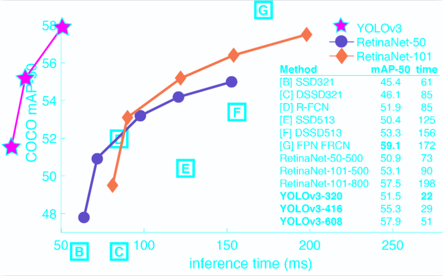
YOLOv3在Pascal Titan X上处理608x608图像速度达到20FPS，在 COCO test-dev 上 mAP@0.5 达到 57.9%，与RetinaNet（FocalLoss论文所提出的单阶段网络）的结果相近，并且速度快4倍.
YOLO v3的模型比之前的模型复杂了不少，可以通过改变模型结构的大小来权衡速度与精度。

2. 改进之处

多尺度预测（类FPN）
更好的基础分类网络（类ResNet）和分类器

分类器-类别预测

YOLOv3不使用Softmax对每个框进行分类

Softmax使得每个框分配一个类别（score最大的一个），而对于Open Images这种数据集，目标可能有重叠的类别标签，因此Softmax不适用于多标签分类。Softmax可被独立的多个logistic分类器替代，且准确率不会下降。分类损失采用binary cross-entropy loss.

多尺度预测

每种尺度预测3个box, anchor的设计方式仍然使用聚类,得到9个聚类中心,将其按照大小均分给3中尺度

尺度1: 在基础网络之后添加一些卷积层再输出box信息.
尺度2: 从尺度1中的倒数第二层的卷积层上采样(x2)再与最后一个16x16大小的特征图相加,再次通过多个卷积后输出box信息.相比尺度1变大两倍.
尺度3: 与尺度2类似,使用了32x32大小的特征图.

基础网络 Darknet-53

仿ResNet, 与ResNet-101或ResNet-152准确率接近,但速度更快.
网络结构如下图所示

YOLOv3在 $mAP^{0.5}$ 及小目标 $AP^S$ 上具有不错的结果,但随着IOU的增大,性能下降,说明YOLOv3不能很好地与ground truth切合.

4. 边框预测

作者尝试了常规的预测方式(Faster R-CNN),然而并不奏效: x,y的偏移作为box的长宽的线性变换
$\begin{cases} \hat{ G } _ { x } = P _ { w } t _ { x } ( P ) + P _ { x } \\ \hat{ G } _ { y } = P _ { h } t _ { y } ( P ) + P _ { y }\\ \hat{ G } _ {w} = P _ { w } e^{t_w(P)}\\ \hat{ G } _ { h } = P _ {h} e^{t_h(P)} \end{cases}$
仍采用之前的logistic方式

  $$\left.\begin{array}{l} { b _ { 2 } = o ( t _ { x } ) + c _ { x } } \\ { b _ { y } = o ( t _ { y } ) + c _ { y } } \\ { b _ { w } = p _ { w } e ^ { t_w } } \\  { b _ { w } = p _ { h } e ^ { t_h } } \end{array}\right. $$

其中 $c_x,c_y$ 是网格的坐标偏移量 $p_w,p_h$ 是预设的anchor box的边长.最终得到的边框坐标值是 $b_{x,y,w,h}$ ,而网络学习目标是 $t_{x,y,w,h}$

5. 优缺点

优点

快速,pipline简单.
背景误检率低。
通用性强。YOLO对于艺术类作品中的物体检测同样适用。它对非自然图像物体的检测率远远高于DPM和RCNN系列检测方法

相比RCNN系列物体检测方法，YOLO具有以下缺点

识别物体位置精准性差
召回率低。在每个网格中预测固定数量的bbox这种约束方式减少了候选框的数量

YOLO v.s. Faster R-CNN

6. 统一网络

YOLO没有显示求取region proposal的过程。Faster R-CNN中尽管RPN与fast rcnn共享卷积层，但是在模型训练过程中，需要反复训练RPN网络和fast rcnn网络.
相对于R-CNN系列的"看两眼",YOLO只需要Look Once.
YOLO统一为一个回归问题
R-CNN将检测结果分为两部分求解：物体类别（分类问题），物体位置即bounding box（回归问题）

二、数据集

1. VOC数据集 Pascal VOC（Pascal Visual Object Classes）

VOC数据集是目标检测经常用的一个数据集，从05年到12年都会举办比赛（比赛有task： Classification 、Detection（将图片中所有的目标用bounding box框出来）、 Segmentation（将图片中所有的目标分割出来）、Person Layout）

VOC2007：中包含9963张标注过的图片，由train/val/test三部分组成，共标注出24,640个物体。 VOC2007的test数据label已经公布，之后的没有公布（只有图片，没有label）。

VOC2012：对于检测任务，VOC2012的trainval/test包含08-11年的所有对应图片。 trainval有11540张图片共27450个物体。对于分割任务， VOC2012的trainval包含07-11年的所有对应图片， test只包含08-11。trainval有 2913张图片共6929个物体。

这些物体一共分为20类

Person: person
Animal: bird, cat, cow, dog, horse, sheep
Vehicle: aeroplane, bicycle, boat, bus, car, motorbike, train
Indoor: bottle, chair, dining table, potted plant, sofa, tv/monitor

文件夹结构

Annotation文件夹存放的是xml文件，该文件是对图片的解释，每张图片都对于一个同名的xml文件。xml主要介绍了对应图片的基本信息，如来自那个文件夹、文件名、来源、图像尺寸以及图像中包含哪些目标以及目标的信息等等

  <annotation>
      <folder>VOC2007</folder>
      <filename>000005.jpg</filename>#文件名
      <source>#文件来源
          <database>The VOC2007 Database</database>
          <annotation>PASCAL VOC2007</annotation>
          <image>flickr</image>
          <flickrid>325991873</flickrid>
      </source>
      <owner>
          <flickrid>archintent louisville</flickrid>
          <name>?</name>
      </owner>
      <size>#文件尺寸，包括长、宽、通道数
          <width>500</width>
          <height>375</height>
          <depth>3</depth>
      </size>
      <segmented>0</segmented>#是否用于分割
      <object>#检测目标
          <name>chair</name>#目标类别
          <pose>Rear</pose>#摄像头角度
          <truncated>0</truncated>#是否被截断，0表示完整
          <difficult>0</difficult>#目标是否难以识别，0表示容易识别
          <bndbox>#bounding-box
              <xmin>263</xmin>
              <ymin>211</ymin>
              <xmax>324</xmax>
              <ymax>339</ymax>
          </bndbox>
      </object>
      <object>#检测到的多个物体
          <name>chair</name>
          <pose>Unspecified</pose>
          <truncated>0</truncated>
          <difficult>0</difficult>
          <bndbox>
              <xmin>165</xmin>
              <ymin>264</ymin>
              <xmax>253</xmax>
              <ymax>372</ymax>
          </bndbox>
      </object>
      <object>#检测到的多个物体
          <name>chair</name>
          <pose>Unspecified</pose>
          <truncated>1</truncated>
          <difficult>1</difficult>
          <bndbox>
              <xmin>5</xmin>
              <ymin>244</ymin>
              <xmax>67</xmax>
              <ymax>374</ymax>
          </bndbox>
      </object>
      <object>
          <name>chair</name>
          <pose>Unspecified</pose>
          <truncated>0</truncated>
          <difficult>0</difficult>
          <bndbox>
              <xmin>241</xmin>
              <ymin>194</ymin>
              <xmax>295</xmax>
              <ymax>299</ymax>
          </bndbox>
      </object>
      <object>#检测到的多个物体
          <name>chair</name>
          <pose>Unspecified</pose>
          <truncated>1</truncated>
          <difficult>1</difficult>
          <bndbox>
              <xmin>277</xmin>
              <ymin>186</ymin>
              <xmax>312</xmax>
              <ymax>220</ymax>
          </bndbox>
      </object>
  </annotation>

ImageSets文件夹存放的是txt文件，这些txt将数据集的图片分成了各种集合。如Main下的train.txt中记录的是用于训练的图片集合

Action下存放的是人的动作（例如running、jumping等等，这也是VOC challenge的一部分）
Layout下存放的是具有人体部位的数据（人的head、hand、feet等等，这也是VOC challenge的一部分）
Main下存放的是图像物体识别的数据，总共分为20类。(train、val、trainval的txt)
- _train中存放的是训练使用的数据，每一个class的train数据都有5717个。
- _val中存放的是验证结果使用的数据，每一个class的val数据都有5823个。
- _trainval将上面两个进行了合并，每一个class有11540个。
  - -1代表负样本，1代表正样本
Segmentation下存放的是可用于分割的数据。

JPEGImages文件夹存放的是数据集的原图片

SegmentationClass以及SegmentationObject文件夹存放的都是图片，且都是图像分割结果图
- SegmentationClass 这里面包含了2913张图片，每一张图片都对应JPEGImages里面的相应编号的图片。这里面的图片的像素颜色共有20种，对应20类物体。比如所有飞机都会被标为红色
- SegmentationObject
  - 这里面同样包含了2913张图片，图片编号都与Class里面的图片编号相同。这里面的图片和Class里面图片的区别在于，这是针对Object的。在Class里面，一张图片里如果有多架飞机，那么会全部标注为红色。而在Object里面，同一张图片里面的飞机会被不同颜色标注出来

2. COCO数据集 Microsoft COCO(Common Objects in Context)

主要特点

（1）Object segmentation
（2）Recognition in Context
（3）Multiple objects per image
（4）More than 300,000 images
（5）More than 2 Million instances
（6）80 object categories
（7）5 captions per image
（8）Keypoints on 100,000 people

主要解决3个问题：目标检测，目标之间的上下文关系，目标的2维上的精确定位。

COCO通过大量使用Amazon Mechanical Turk来收集数据。COCO数据集现在有3种标注类型：object instances（目标实例）, object keypoints（目标上的关键点）, 和image captions（看图说话），使用JSON文件存储。

基本的JSON结构体类型
共享这些基本类型：info、image、license

annotation类型则呈现出了多态

   
   {
       "info": info,
       "licenses": [license],
       "images": [image],
       "annotations": [annotation],
   }
       
   info{
       "year": int,
       "version": str,
       "description": str,
       "contributor": str,
       "url": str,
       "date_created": datetime,
   }
   license{
       "id": int,
       "name": str,
       "url": str,
   } 
   image{
       "id": int,
       "width": int,
       "height": int,
       "file_name": str,
       "license": int,
       "flickr_url": str,
       "coco_url": str,
       "date_captured": datetime,
   }

info类型

   
   "info":{
   	"description":"This is stable 1.0 version of the 2014 MS COCO dataset.",
   	"url":"http:\\mscoco.org",
   	"version":"1.0","year":2014,
   	"contributor":"Microsoft COCO group",
   	"date_created":"2015-01-27 09:11:52.357475"
   },

Images是包含多个image实例的数组

        
        {
        	"license":3,
        	"file_name":"COCO_val2014_000000391895.jpg",
        	"coco_url":"http:\\mscoco.org\images\391895",
        	"height":360,"width":640,"date_captured":"2013-11-14 11:18:45",
        	"flickr_url":"http:\\farm9.staticflickr.com\8186\8119368305_4e622c8349_z.jpg",
        	"id":391895
        },

licenses是包含多个license实例的数组


{
	"url":"http:\\creativecommons.org\licenses\by-nc-sa\2.0\",
	"id":1,
	"name":"Attribution-NonCommercial-ShareAlike License"
},

3. Object Instance 类型的标注格式

整体JSON文件格式

{    
    "info": info,      
    "licenses": [license],    
    "images": [image],      
    "annotations": [annotation],    
    "categories": [category]
   }

images数组元素的数量等同于划入训练集（或者测试集）的图片的数量；
annotations数组元素的数量等同于训练集（或者测试集）中bounding box的数量；
categories数组元素的数量为80（2017年）；

annotations字段

包含多个annotation实例的一个数组，annotation类型本身又包含了一系列的字段，如这个目标的category id和segmentation mask。segmentation格式取决于这个实例是一个单个的对象（即iscrowd=0，将使用polygons格式）还是一组对象（即iscrowd=1，将使用RLE格式）。如下所示：

   annotation{
       "id": int,    
       "image_id": int,
       "category_id": int,
       "segmentation": RLE or [polygon],
       "area": float,
       "bbox": [x,y,width,height],
       "iscrowd": 0 or 1,
   }

4. polygon格式

按照相邻的顺序两两组成一个点的xy坐标，如果有n个数（必定是偶数），那么就是n/2个点坐标。下面就是一段解析polygon格式的segmentation并且显示多边形的示例代码：

     import numpy as np
     import matplotlib.pyplot as plt
     import matplotlib
     from matplotlib.patches import Polygon
     from matplotlib.collections import PatchCollection
     fig, ax = plt.subplots()
     polygons = []
     num_sides = 100
     gemfield_polygons = [[125.12, 539.69, 140.94, 522.43......]]
     gemfield_polygon = gemfield_polygons[0]
     max_value = max(gemfield_polygon) * 1.3
     gemfield_polygon = [i * 1.0/max_value for i in gemfield_polygon]
     poly = np.array(gemfield_polygon).reshape((int(len(gemfield_polygon)/2), 2))
     polygons.append(Polygon(poly,True))
     p = PatchCollection(polygons, cmap=matplotlib.cm.jet, alpha=0.4)
     colors = 100*np.random.rand(1)
     p.set_array(np.array(colors))
     ax.add_collection(p)
     plt.show()

如果iscrowd=1，那么segmentation就是RLE格式(segmentation字段会含有counts和size数组)，在json文件中gemfield挑出一个这样的例子，如下所示

segmentation : 
{
  u'counts': [272, 2, 4, 4, 4, 4, 2, 9, 1, 2, 16, 43, 143, 24......], 
  u'size': [240, 320]
}

categories字段
categories是一个包含多个category实例的数组，而category结构体描述如下：

{
   "id": int,
   "name": str,
   "supercategory": str,
}

5. Object Keypoint 类型的标注格式

整体JSON文件格式

{
   "info": info,
   "licenses": [license],
   "images": [image],
   "annotations": [annotation],
   "categories": [category]
}

annotations字段

annotation{
    "keypoints": [x1,y1,v1,...],
    "num_keypoints": int,
    "id": int,
    "image_id": int,
    "category_id": int,
    "segmentation": RLE or [polygon],
    "area": float,
    "bbox": [x,y,width,height],
    "iscrowd": 0 or 1,
 }

包含了Object Instance中annotation结构体的所有字段，加上2个额外的字段。新增的keypoints是一个长度为3*k的数组，其中k是category中keypoints的总数量。每一个keypoint是一个长度为3的数组，第一和第二个元素分别是x和y坐标值，第三个元素是个标志位v，v为0时表示这个关键点没有标注（这种情况下x=y=v=0），v为1时表示这个关键点标注了但是不可见（被遮挡了），v为2时表示这个关键点标注了同时也可见。

categories字段

{
  "id": int,
  "name": str,
  "supercategory": str,
  "keypoints": [str],
  "skeleton": [edge]
}

6. Image Caption的标注格式

整体JSON文件格式

{
    "info": info,
    "licenses": [license],
    "images": [image],
    "annotations": [annotation]
}

annotations字段

annotation{
    "id": int,
    "image_id": int,
    "caption": str
  }

7. PaddlePaddle 数据集

默认所有的数据都是直接下载到目录'~/.cache/paddle/dataset'
Paddle来指定别的位置数据集

 import paddle 
 import paddle.fluid as fluid
 from paddle.dataset import mnist
 import matplotlib.pyplot as plt
 
 train_data = mnist.train()
 test_data = mnist.test()

paddle返回的是一个方法！！！（这个方法的返回值是一个generator！！！）generator是一个由tuple组成的，且tuple第一个元素为numpy.ndarray, 第二个元素是一个整数

数据进行打乱排序

shuffle

paddle.reader的shuffle函数提供了这个功能，它的第一个参数是从dataset得到的返回generator的函数，第二个参数是每次进行shuffle的数据量。这里的shuffle跟我们日常理解的shuffle还不太一样，它是加载一定数量的数据（我们第二个参数），然后进行shuffle后输出，接着继续进行下一批数据shuffle。如果要全量数据进行shuffle，只要第二个参数大于所有数据总量即可。最后返回的是一个无参函数，函数返回的是一个generator
paddle.reader.shuffle(mnist.train(), buf_size=500)

batch

paddle.batch把数据封装成输出一个一个Batch的形式。第一个参数是无参函数（与dataset和shuffle返回的一样）, 第二个参数是batch的大小。至于batch函数直接放在paddle下面这一层还是挺让我困惑的，我觉得这个函数应该是放在reader里面比较合适。当然啦，这个函数的返回值还是跟前面几个方法一样，都是一个无参函数，其返回值是一个generator

batch_loader = paddle.batch(mnist.train(), batch_size=10)
first_batch = list(batch_loader())[0]
print(type(first_batch))
print(type(first_batch[0]))

batch之后最终数据的是以一个list的方式返回，list大小即为batch大小。

自己的数据集转化为VOC数据集

voc数据集格式

└── VOCdevkit     #根目录
    └── VOC2017   
        ├── Annotations        #存放xml文件，与JPEGImages中的图片一一对应，解释图片的内容等等
        ├── ImageSets          
        │   ├── Action
        │   ├── Layout
        │   ├── Main├── train.txt#存放文件名
        │			├── val.txt
        │			└── test.txt
        │   └── Segmentation
        ├── JPEGImages         #存放源图片
        ├── label_list.txt#存放bbox标签
        ├── train.txt#JPEGImages图片路径与Annotations标签路径应
        ├── val.txt
        └── test.txt

label_list.txt——bbox类别
train.txt
- ImageSets /Main/train.txt,另一个最直接在主目录下

import os
import json
import cv2
import random
 
\# voc格式最后储存位置
voc_format_save_path = r'/home/aistudio/PaddleDetection/dataset/People/ImageSets/Main/train.txt'
\# yolo格式的注释文件，上文有格式
yolo_format_annotation_path = r'/home/aistudio/PaddleDetection/dataset/peopledetection/train.json'
\#另一个train保存路径
train_path = r'/home/aistudio/PaddleDetection/dataset/People/train.txt'

\#判断文件是否存在,path为文件路径

if os.path.exists(voc_format_save_path):
    \#删除文件,path为文件路径
    os.remove(voc_format_save_path)
if os.path.exists(train_path):
    \#删除文件,path为文件路径
    os.remove(train_path)


\# 前面都造好了基础(为了和coco一致，其实很多都用不到的)，现在开始解析自己的数据
f = open(yolo_format_annotation_path,encoding='utf-8')
content = json.load(f)

file = open(voc_format_save_path,'a')
for j in range(len(content['annotations'])):
    img_path=content['annotations'][j]['name']
    img_name = os.path.basename(img_path)
    (img_name, extension) = os.path.splitext(img_name)
    img_name=img_name+'\n'
    file.write(img_name)
file.close()
print('保存成功1')

file2 = open(train_path,'a')
for j in range(len(content['annotations'])):
    img_path=content['annotations'][j]['name']
    img_name = os.path.basename(img_path)
    (img_name1, extension) = os.path.splitext(img_name)
    name='JPEGImages/'+str(img_name)+' '+'Annotations/'+str(img_name1)+'.xml\n'
    file2.write(name)
file2.close()
print('保存成功2')

生成.xml文件

import os, sys
import glob
from PIL import Image
import json
import cv2
import random
 
label_lists = []
img_lists = []
src_label_dir = '/home/aistudio/PaddleDetection/dataset/peopledetection/train.json'                           ###指向自己数据集的labelTxt文件夹
out_xml_dir = '/home/aistudio/PaddleDetection/dataset/People/Annotations/'  ###指向voc数据集的Annotations文件夹

f = open(src_label_dir,encoding='utf-8')
content = json.load(f)
for j in range(len(content['annotations'])):
    content['annotations'][j]['name'] = content['annotations'][j]['name'].lstrip('stage1').lstrip('/')
    img_path = content['annotations'][j]['name']
    img_name = os.path.basename(img_path)
    (img_name, extension) = os.path.splitext(img_name)
    \# 因为需要width和height,而我得yolo文件里没有，所以我还得读图片，很烦
    \# 我就用opencv读取了,当然用其他库也可以
    \# 别把图片路径搞错了，绝对路径和相对路径分清楚！
    img_path = os.path.join('/home/aistudio/',img_path)
    height,width = cv2.imread(img_path).shape[:2]

    \# write in xml file
    \# os.mknod(src_xml_dir + '/' + img + '.xml')
    xml_file = open((out_xml_dir + '/' + img_name + '.xml'), 'w')
    xml_file.write('<annotation>\n')
    xml_file.write('    <folder>VOC2007</folder>\n')
    xml_file.write('    <filename>' + str(img_name) + '.jpg' + '</filename>\n')    ###若准备的图片为jpg格式则将png替换为jpg
    xml_file.write('    <path>' + str(img_path) + '.jpg' + '</path>\n')    ###若准备的图片为jpg格式则将png替换为jpg
    xml_file.write('    <size>\n')
    xml_file.write('        <width>' + str(width) + '</width>\n')
    xml_file.write('        <height>' + str(height) + '</height>\n')
    xml_file.write('        <depth>3</depth>\n')
    xml_file.write('    </size>\n')
    xml_file.write('    <segmented>0</segmented>\n')
    for bbox in  content['annotations'][j]['annotation']:
        xmin=bbox['x']
        ymin=bbox['y']
        xmax=bbox['x']+bbox['w']
        ymax=bbox['y']+bbox['h']
        gt_label = content['annotations'][j]['type']
        xmin,ymin,xmax,ymax= int(xmin),int(ymin),int(xmax),int(ymax)
    

        xml_file.write('    <object>\n')
        xml_file.write('        <name>'+str(gt_label)+'</name>\n')
        xml_file.write('        <pose>Unspecified</pose>\n')
        xml_file.write('        <truncated>0</truncated>\n')
        xml_file.write('        <difficult>0</difficult>\n')
        xml_file.write('        <bndbox>\n')
        xml_file.write('            <xmin>'+str(xmin)+'</xmin>\n')
        xml_file.write('            <ymin>'+str(ymin)+'</ymin>\n')
        xml_file.write('            <xmax>'+str(xmax)+'</xmax>\n')
        xml_file.write('            <ymax>'+str(ymax)+'</ymax>\n')
        xml_file.write('        </bndbox>\n')
        xml_file.write('    </object>\n')
    xml_file.write('</annotation>')    
    xml_file.close()

把图片文件copy到JPEGImages文件夹下，直接使用Linux命令cp -r

Magician0619

关注

1
点赞
踩
5

收藏

觉得还不错? 一键收藏
打赏
0
评论
YOLO学习总结与数据集制作

文章目录一、YOLOV3概述1. YOLOV3特点2. 改进之处4. 边框预测5. 优缺点6. 统一网络二、数据集1. VOC数据集 Pascal VOC（Pascal Visual Object Classes）2. COCO数据集 Microsoft COCO(Common Objects in Context)3. Object Instance 类型的标注格式4. polygon格式5....
复制链接

扫一扫