


知识要点
- tensorflow 中的代码做了优化, 速度会快一些.
- np.where(condition,x,y): 当where内有三个参数时,第一个参数表示条件,当条件成立时where方法返回x,当条件不成立时where返回y.
- 判断是否相等: tf.greater_equal(a, b) # ==
- 求导: tf.GradientTrape
- tensor 变量定义: tf.Variable(2.0)
- 常量定义: x1 = tf.constant(2.0)
- x_train, x_valid, y_train, y_valid = train_test_split(x_train_all, y_train_all, random_state = 11) # 数据拆分, 从x_train_all中切割出训练数据和校验数据
- 标准化处理: train_scaled = scaler.fit_transform(x_train) # scaler = StandardScaler()
- 梯度更新:
# 计算损失函数中参数的梯度,
with tf.GradientTape() as tape:
    grads = tape.gradient(loss, model.variables)
    # 更新
    grads_and_vars = zip(grads, model.variables)
optimizer.apply_gradients(grads_and_vars)- 合并数据矩阵: train_data = np.c_[x_train_scaled, y_train]
- 将元素放置到一起: tf.stack(parsed_fields)
- callbacks = [keras.callbacks.EarlyStopping(patience = 5, min_delta = 1e-2)] # fit 中的callback设置
- matplotlib 画图:
- pd.DataFrame(history.history).plot(figsize = (8, 5)) # 设置图片大小
- plt.grid(True) # 画背景
- plt.gca().set_ylim(0, 1.5) # 设置y 轴
- plt.show() # 画图
1. python 函数转换为 tensorflow 中的函数
- tensorflow 中的代码做了优化, 速度会快一些
- 判断是否相等: tf.greater_equal(a, b) # ==
- tf.where()定义如下:
- tf.where(condition, x=None, y=None,name=None)
- condition: 一个 tensor,数据类型为tf.bool/bool类型
- condition, x, y 相同维度,condition是bool型值,True/False
- 如果x、y均为空,那么返回condition中值为True的位置组成的Tensor:例如:x就是condition,y是返回值。或者说,是condition中元素为True对应的索引。
- 如果x、y不为空,那么x、y必须有相同的形状。如果x、y是标量,那么condition参数也必须是标量。如果x、y是向量,那么condition必须和x的第一维有相同的形状或者和x形状一致。
- 返回值:如果x、y不为空的话,返回值和x、y有相同的形状,如果condition对应位置值为True那么返回Tensor对应位置为x的值,否则为y的值.
from tensorflow import keras
import numpy as np
import pandas
import matplotlib.pyplot as plt
import tensorflow as tf
import time

# 如何把python函数转化为TensorFlow 中的函数
# tensorflow 中的代码做了优化, 速度会快一些
# elu z > 0? scale * z
def scaled_elu(z, scale = 1.0, alpha = 1.0):
    is_positive = tf.greater_equal(z, 0.0)
    # np.where
    return scale * tf.where(is_positive, z, alpha * tf.nn.elu(z))
1.1 标量设置
print(scaled_elu(tf.constant(-3.0)))     # 标量
'''tf.Tensor(-0.95021296, shape=(), dtype=float32)'''
1.2 向量设置
print(scaled_elu(tf.constant([-3.0, -2.5])))     # 向量
'''tf.Tensor([-0.95021296 -0.917915  ], shape=(2,), dtype=float32)'''
1.3 定义函数
scaled_elu_tf = tf.function(scaled_elu)
scaled_elu_tf

print(scaled_elu_tf(tf.constant(-3.0)))
print(scaled_elu_tf(tf.constant([-3.0, -2.5])))![]()
- 两种方式进行比较:
- 方式一: 用自定义的函数实现数据转换为tensor, 耗时: 12s
%%time
%timeit scaled_elu(tf.random.normal((1000, 1000))) 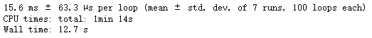
- 方式二: 用tensorlow 转换为tensor, 耗时: 10s # 效率还是高一些
%%time
%timeit scaled_elu_tf(tf.random.normal((1000, 1000)))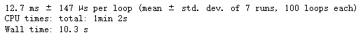
scaled_elu_tf.python_function is scaled_elu # true1.4 函数定义
- AutoGraph:将 Python 控制流转换为 TensorFlow 计算图
- @tf.function 使用名为 AutoGraph 的机制将函数中的 Python 控制流语句转换成 TensorFlow 计算图中的对应节点,使用 tf.autograph 模块的低层 API tf.autograph.to_code 将函数 square_if_positive 转换成 TensorFlow 计算图
# tf.function 装饰器的写法
# 1 + 1/2 + 1/2^2 + .... + 1/2^n = 2
@tf.function
def converge_to_2(n_iters):
    total = tf.constant(0.)
    increment = tf.constant(1.)
    for _ in range(n_iters):
        total += increment
        increment /= 2.0
    return total

converge_to_2(24)
'''<tf.Tensor: shape=(), dtype=float32, numpy=1.9999999>'''
from IPython.display import display, Markdown
# 展示TensorFlow内部的计算代码
def display_tf_code(func):
code = tf.autograph.to_code(func)
display(Markdown('```python\n{}\n```'.format(code)))
display_tf_code(scaled_elu)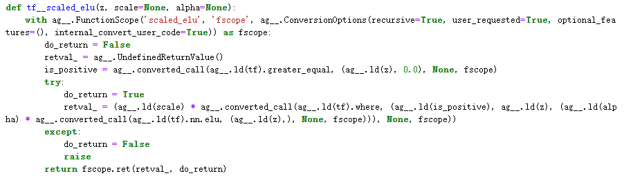
# 函数操作的是TensorFlow的变量, 那么要把变量定义在函数外面
var = tf.Variable(0.)
@tf.function
def add_21():
    return var.assign_add(21)  # 21
print(add_21())     # tf.Tensor(21.0, shape=(), dtype=float32)
2 手动实现微分
2.1 微分
# 手动微分, 求导
def f(x):
    return 3. * x** 2 + 2. * x - 1    # 3 * x^2 + 2 *x - 1
# 近似求导: (f(x + x1) - f(x - eps))/2x1
def approxmate_derivative(f, x, eps = 1e-3):
    return (f(x + eps) - f(x -eps))/ (2. * eps)   # 斜率:f(x)'

# 两个未知数, 求偏导
def g(x1, x2):
    return (x1 + 5) * (x2 ** 2)   # (x1+5)*x2^2
# 分别求g 对x1, 和x2的偏导
def approxmate_gradient(g, x1, x2, eps = 1e-3):
    dg_x1 = approxmate_derivative(lambda x: g(x, x2), x1, eps)
    dg_x2 = approxmate_derivative(lambda x: g(x1, x), x2, eps)
    return dg_x1, dg_x2
approxmate_gradient(g, 2, 3)  # (8.999999999993236, 41.999999999994486)
# tf.GradientTrape 来求导
x1 = tf.Variable(2.0)
x2 = tf.Variable(3.0)
with tf.GradientTape(persistent = True) as tape:
z = g(x1, x2)
dz_x1 = tape.gradient(z, x1)
print(dz_x1) # tf.Tensor(9.0, shape=(), dtype=float32)
dz_x2 = tape.gradient(z, x2)
print(dz_x2) # tf.Tensor(42.0, shape=(), dtype=float32)
del tape 2.2 变量求导
x1 = tf.Variable(2.0)  # 变量
x2 = tf.Variable(3.0)
with tf.GradientTape() as tape:
    z = g(x1, x2)

dz_x1x2 = tape.gradient(z, [x1, x2])
print(dz_x1x2)
'''[<tf.Tensor: shape=(), dtype=float32, numpy=9.0>,
    <tf.Tensor: shape=(), dtype=float32, numpy=42.0>]'''
2.3 常量求导
# 常量求导
x1 = tf.constant(2.0)  # 常量, 需要使用watch去关注它, 然后才可以求导
x2 = tf.constant(3.0)
with tf.GradientTape() as tape:
    tape.watch(x1)
    tape.watch(x2)
    z = g(x1 ,x2)

# 默认是不会对常量求导.
dz_x1x2 = tape.gradient(z, [x1, x2])
print(dz_x1x2)
'''[<tf.Tensor: shape=(), dtype=float32, numpy=9.0>,
    <tf.Tensor: shape=(), dtype=float32, numpy=42.0>]'''
2.4 导数累加
x = tf.Variable(5.0)
with tf.GradientTape() as tape:
    z1 = 3 * x
    z2 = x ** 2
# 会把导数累加起来
tape.gradient([z1, z2], x)  # <tf.Tensor: shape=(), dtype=float32, numpy=13.0>
2.5 二阶导数
# 二阶导数 嵌套tf.gradientTape
x1 = tf.Variable(2.0)  # 变量
x2 = tf.Variable(3.0)
with tf.GradientTape(persistent = True) as outer_tape:
    with tf.GradientTape(persistent = True) as inner_tape:
        z = g(x1 ,x2)
    # 求一阶导数
    inner_grads = inner_tape.gradient(z, [x1, x2])  # graddent  导数

# 对一阶导数求导,
out_grads=[outer_tape.gradient(inner_grad,[x1, x2])for inner_grad in inner_grads]
print(out_grads)
'''[[None, <tf.Tensor: shape=(), dtype=float32, numpy=6.0>], [<tf.Tensor: shape=(),
dtype=float32,numpy=6.0>, <tf.Tensor: shape=(), dtype=float32, numpy=14.0>]]'''
del inner_tape, outer_tape
2.6 梯度下降
# 使用tf.GradientTape 实现梯度下降
learning_rate = 0.1
x = tf.Variable(0.0)
for _ in range(100):
    with tf.GradientTape() as tape:
        z = f(x)
    dz_dx = tape.gradient(z, x)
    x.assign_sub(learning_rate * dz_dx)  # x -= learning_rate * dzdx
print(x)  # <tf.Variable 'Variable:0' shape=() dtype=float32, numpy=-0.3333333>
2.7 结合optimizer 实现梯度下降
# 使用tf.GradientTape 实现梯度下降
# 结合optimizer 去实现梯度下降
learning_rate = 0.1
x = tf.Variable(0.0)
optimizer = keras.optimizers.SGD(lr = learning_rate)
for _ in range(100):
    with tf.GradientTape() as tape:
        z = f(x)
    dz_dx = tape.gradient(z, x)
    optimizer.apply_gradients([(dz_dx, x)])
print(x)  # <tf.Variable 'Variable:0' shape=() dtype=float32, numpy=-0.3333333>
3 手动实现训练过程
3.1 导入加利福尼亚州房价
from sklearn.datasets import fetch_california_housing
from sklearn.model_selection import train_test_split
# 切割数据
housing = fetch_california_housing()
x_train_all, x_test, y_train_all, y_test = train_test_split(housing.data, housing.target, random_state = 7)
# 从x_train_all中切割出训练数据和校验数据
x_train, x_valid, y_train, y_valid = train_test_split(x_train_all, y_train_all, random_state = 11)
print(x_train.shape, y_train.shape)  # (11610, 8) (11610,)
print(x_valid.shape, y_valid.shape)  # (3870, 8) (3870,)
print(x_test.shape, y_test.shape)    # (5160, 8) (5160,)
3.2 标准化处理训练数据
# 标准化处理
from sklearn.preprocessing import StandardScaler, MinMaxScaler
scaler = StandardScaler()
# 对之前部分trainData进行fit的整体指标,对剩余的数据(testData)使用同样的均值、方差
# 最大最小值等指标进行转换transform(testData),从而保证train、test处理方式相同
x_train_scaled = scaler.fit_transform(x_train)
x_valid_scaled = scaler.transform(x_valid)
x_test_scaled = scaler.transform(x_test)
3.3 模型训练 (手动实现fit部分)
# 遍历数据集  # 自动求导  epoch 验证集
batch_size = 32
steps_per_epoch = len(x_train_scaled) // batch_size
optimizer = keras.optimizers.SGD()
metric = keras.metrics.MeanSquaredError()

def random_batch(x, y, batch_size = 32):
    idx = np.random.randint(0, len(x), size = batch_size)
    return x[idx], y[idx]

# 定义网络
model = keras.models.Sequential([
    # input_dim是传入数据, input_shape一定要是元组
    keras.layers.Dense(128, activation = 'relu', input_shape = x_train.shape[1:]),
    keras.layers.Dense(64, activation = 'tanh'),
    keras.layers.Dense(1)])

epochs = 20
callbacks = []
# 自定义训练过程
for epoch in range(epochs):
    # 每次epoch需要重置评估指标
    metric.reset_states()
    for step in range(steps_per_epoch):
        x_batch, y_batch = random_batch(x_train_scaled, y_train, batch_size)
        # 求导
        with tf.GradientTape() as tape:
            y_pred = model(x_batch)
            y_pred = tf.squeeze(y_pred, 1)  # 传参中保证形状和y_train形状一致
            # 计算损失
            loss = keras.losses.mean_squared_error(y_batch, y_pred)
            metric(y_batch, y_pred)

        # 计算损失函数中参数的梯度,
        grads = tape.gradient(loss, model.variables)
        # 更新
        grads_and_vars = zip(grads, model.variables)
        optimizer.apply_gradients(grads_and_vars)
        print('epoch:', epoch, 'train_mse', metric.result().numpy(), end = '')
        print('\n')
    # 校验一下
    # 每个epoch 去计算校验集的效果
    y_valid_pred = model(x_valid_scaled)
    y_pred = tf.squeeze(y_valid_pred, 1)
    valid_loss = keras.losses.mean_squared_error(y_valid, y_valid_pred)
    print('\t', 'valid mse:', valid_loss.numpy())
4 保存和读取CSV文件
4.1 读取文件
from sklearn.datasets import fetch_california_housing
housing = fetch_california_housing()
# 基础数据
x_train_all, x_test, y_train_all, y_test = train_test_split(housing.data, housing.target)
x_train, x_valid, y_train, y_valid = train_test_split(x_train_all, y_train_all)
4.2 读取大数据集
- 如何使用TensorFlow批量读取CSV文件, 然后汇总为一个大的数据集
- 1. 生成CSV文件
- 2. 读取CSV文件
- 3. 解析字段
- 4. 变成dataset
# 生成CSV文件
import os
output_dir = 'generate_csv'
# 如果不存在,则创建目录
if not os.path.exists(output_dir):
    os.mkdir(output_dir)
# 分批读取数据
def save_to_csv(output_dir, data, name_prefix, header = None, n_parts = 10):
    # 生成CSV的文件名
    path_format = os.path.join(output_dir, '{}_{:02d}.csv')
    filenames = []

    for file_idx, row_indices in enumerate(np.array_split(np.arange(len(data)), n_parts)):
        # 每一个CSV的文件名
        part_csv = path_format.format(name_prefix, file_idx)
        filenames.append(part_csv)

        # 取数据, 写入文件
        with open(part_csv, 'wt', encoding = 'utf-8') as f:
            if header is not None:
                f.write(header + '\n')
            # 依次取出数据
            for row_index in row_indices:
                f.write(','.join([repr(col) for col in data[row_index]]))
                f.write('\n')
    return filenames
4.3 合并数据
# 依次生成训练数据. 校验数据. 测试数据的CSV文件
# 把样本数据和对应数据合并到一起
train_data = np.c_[x_train_scaled, y_train]
valid_data = np.c_[x_valid_scaled, y_valid]
test_data = np.c_[x_test_scaled, y_test]- 特征拼接
# 生成抬头
header_cols = housing.feature_names + ['MedianHouseValue']
header_str = ','.join(header_cols)
header_str
'''MedInc,HouseAge,AveRooms,AveBedrms,Population,AveOccup,Latitude,Longitude,
MedianHouseValue 医疗,房屋年龄,客房,床位,人口,住房占用,纬度,经度,价值中位数'''- 保存文件
# 生成CSV文件
train_filenames=save_to_csv(output_dir, train_data,'train', header_str, n_parts = 20)
valid_filenames=save_to_csv(output_dir, valid_data,'valid', header_str, n_parts = 20)
test_filenames = save_to_csv(output_dir, test_data, 'test', header_str, n_parts = 20)
4.4 读取CSV文件
# tf.dataset.list_files 可以从文件名列表中生成dataset
filename_dataset = tf.data.Dataset.list_files(train_filenames)
for filename in filename_dataset:
    print(filename)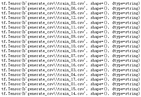
# 对filename_dataset 中的每一个文件进行读取
n_readers = 5
# skip(1), 跳过第一行
dataset = filename_dataset.interleave(lambda filename: tf.data.TextLineDataset(filename).skip(1),
                                      cycle_length = n_readers)
for line in dataset.take(15):
    print(line.numpy())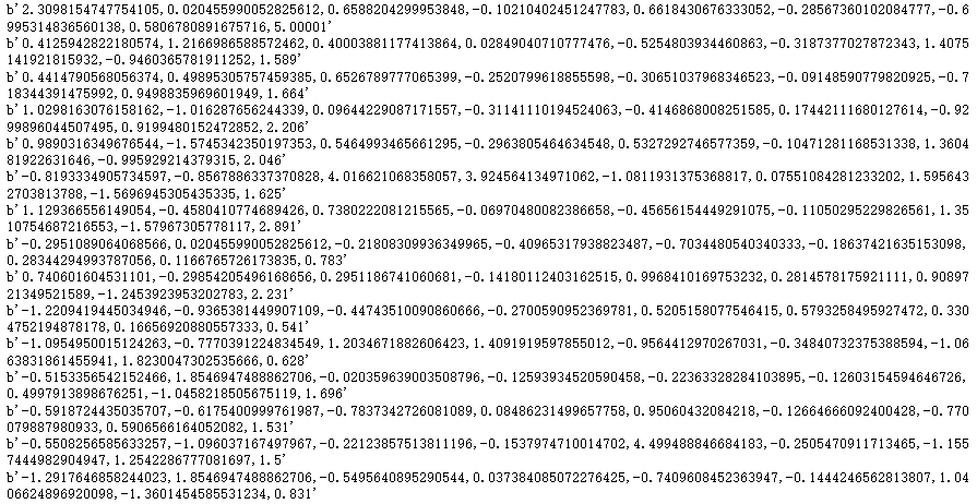
- 解析CSV
# 解析csv
# tensorflow中解析CSV中的文件的api, tf.io.decode_csv()
sample_str = '1,2,3,4,5'
# 字段对应的类型
# 注意事项, csv中的字段个数和record_defaults中的个数必须数量一致
record_defaults = [tf.constant(0, dtype = tf.int32)] * 5
parsed_fields = tf.io.decode_csv(sample_str, record_defaults)
# parsed_filelds = tf.io.decode_csv(sample_str, record_defaults)
print(parsed_fields)
# 将元素放置到一起, tf.stack
tf.stack(parsed_fields) # <tf.Tensor:shape=(5,),dtype=int32,numpy=array([1,2,3,4,5])>![]()
- 封装解析
# 封装解析一行csv的函数
def parse_csv_line(line, n_fields = 9):
    record_defaults = [tf.constant(np.nan)] * n_fields
    parsed_fields = tf.io.decode_csv(line, record_defaults)
    x = tf.stack(parsed_fields[0:-1])
    y = tf.stack(parsed_fields[-1:])
    return x, y
parse_csv_line(b'-0.4228275640611027,0.6554110272436566,-0.017487894261755055,-0.1076332693171028,-0.4857755004630467,-0.0022432283128525714,-1.4069801142822567,1.2347344206850313,1.287')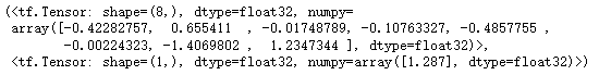
- 整体封装
# 将功能封装到一起
def csv_reader_dataset(filenames, n_readers= 5, batch_size = 32, n_parse_threads = 5,
                       shuffle_buffer_size = 10000):
    dataset = tf.data.Dataset.list_files(filenames)
    # 无限重复
    dataset = dataset.repeat()
    # 对每一行数据进行读取
    dataset = dataset.interleave(lambda filename: tf.data.TextLineDataset(filename).skip(1),
                       cycle_length = n_readers)
    # 打乱数据
    dataset.shuffle(shuffle_buffer_size)
    # 对dataset中的每一个item做操作
    dataset = dataset.map(parse_csv_line, num_parallel_calls = n_parse_threads)
    dataset = dataset.batch(batch_size)
    return dataset

# 看看训练数据效果
train_set = csv_reader_dataset(train_filenames, batch_size= 3)
print(train_set)
for x_batch, y_batch in train_set.take(2):
    print('x:')
    print('***', x_batch)
    print('+++', y_batch)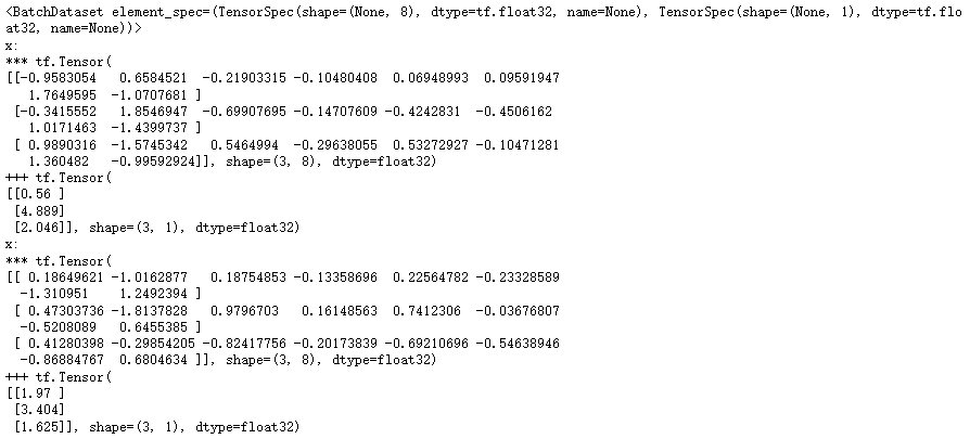
4.5 执行读取并训练
- 读取数据
batch_size = 32
train_set = csv_reader_dataset(train_filenames, batch_size = batch_size)
valid_set = csv_reader_dataset(valid_filenames, batch_size = batch_size)
test_set = csv_reader_dataset(test_filenames, batch_size = batch_size)- 定义模型
# 定义模型
model = keras.models.Sequential([keras.layers.Dense(30, activation = 'relu', input_shape = [8]),
keras.layers.Dense(1)]) 
- 执行训练
model.compile(loss = 'mse', optimizer = 'adam', metrics = ['mse'])
callbacks = [keras.callbacks.EarlyStopping(patience = 5, min_delta = 1e-2)]

history = model.fit(train_set, validation_data= valid_set,
                    # 不指定步数会一直训练
                    steps_per_epoch = 11610// batch_size,
                    validation_steps = 3870// batch_size,
                    epochs = 100,
                    callbacks = callbacks)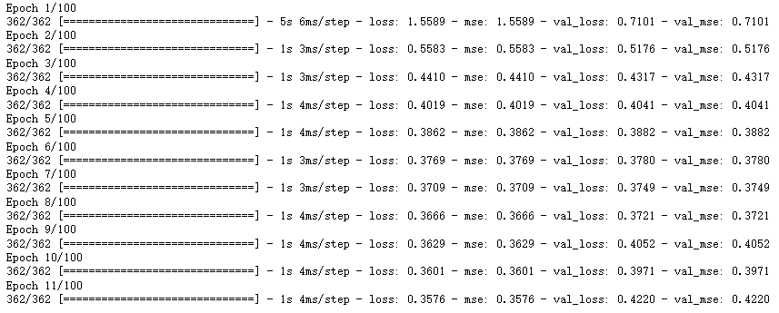
- 提前终止, 执行了early_stop
5 自定义layer
5.1 导包
from tensorflow import keras
import numpy as np
import pandas as pd
import matplotlib.pyplot as plt
5.2 导入数据
from sklearn.datasets import fetch_california_housing
housing = fetch_california_housing()
# 切割数据
# 训练数据, 验证集, 测试数据
from sklearn.model_selection import train_test_split

x_train_all, x_test, y_train_all, y_test = train_test_split(housing.data, housing.target, random_state = 7)
# 从x_train_all中切割出训练数据和校验数据
x_train, x_valid, y_train, y_valid = train_test_split(x_train_all, y_train_all, random_state = 11)

print(x_train.shape, y_train.shape)    # (11610, 8) (11610,)
print(x_valid.shape, y_valid.shape)    # (3870, 8) (3870,)
print(x_test.shape, y_test.shape)      # (5160, 8) (5160,)
5.3 标准化处理
# 标准化处理
from sklearn.preprocessing import StandardScaler,MinMaxScaler
scaler = StandardScaler()
x_train_scaled = scaler.fit_transform(x_train)
x_valid_scaled = scaler.transform(x_valid)
x_test_scaled = scaler.transform(x_test)
5.4 查看layers情况
layer = keras.layers.Dense(30, activation = 'relu', input_shape = (None, 5))
print(layer)   # <keras.layers.core.dense.Dense at 0x2250ed82100>
layer(np.zeros((10, 5)))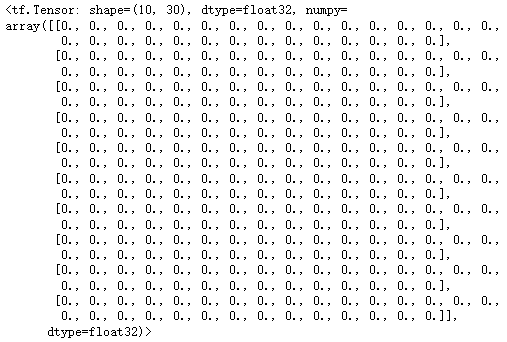
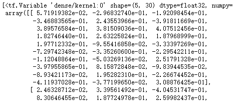
- layer.variables: 可以查看层次中的变量
- layer.trainable_variables: 可以查看可训练的变量
layer.trainable_variables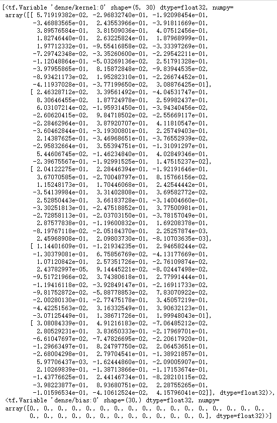
5.5 自定义layer
- 重写layer
# 自定义layer
class CustomizedDenseLayer(keras.layers.Layer):
    def __init__(self, units, activation = None, **kwargs):
        self.units = units
        self.activation = keras.layers.Activation(activation)
        super().__init__(**kwargs)

    def build(self, input_shape):
        '''构建所需要的参数'''
        # None, 8 @ w + b  # w * x + b
        self.kernel = self.add_weight(name = 'kernel', shape = (input_shape[1], self.units),
                        initializer = 'uniform', trainable = True)
        self.bias = self.add_weight(name = 'bias', shape = (self.units,), initializer = 'zeros', trainable = True)
        super().build(input_shape)

    def call(self, x):
        '''完成正向传播'''
        return self.activation(x@ self.kernel + self.bias)
# 通过lambda 函数快速自定义层次
# softplus: log(1 + e^x))
customized_softplus = keras.layers.Lambda(lambda x :tf.nn.softplus(x))
print(customized_softplus)
customized_softplus([-10., -4., 0., 5., 10.])
-
定义模型
# 定义网络  CustomizedDenseLayer
model = keras.models.Sequential([
    # input_dim是传入数据, input_shape一定要是元组
    CustomizedDenseLayer(128, activation = 'relu', input_shape = x_train.shape[1:]),
    customized_softplus,
    CustomizedDenseLayer(64, activation = 'tanh'),
    customized_softplus,
    CustomizedDenseLayer(1)])
model.summary()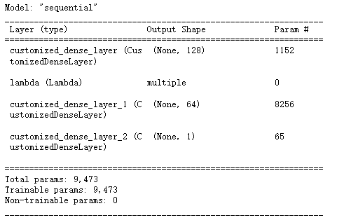
5.6 训练模型
# 配置模型  # epochs 迭代次数
model.compile(loss = 'mean_squared_error', optimizer = 'sgd', metrics = ['mse'])
history = model.fit(x_train_scaled, y_train, validation_data = (x_valid_scaled, y_valid), epochs = 20) 
# 定义画图函数, 看是否过拟合
def plot_learning_curves(history):
    pd.DataFrame(history.history).plot(figsize = (8, 5))
    plt.grid(True)
    plt.gca().set_ylim(0, 1)
    plt.show()
plot_learning_curves(history)
6 自定义损失函数
- 自定义损失
# 自定义损失函数
def customized_mse(y_true, y_pred):
    return tf.reduce_mean(tf.square(y_pred - y_true))

model.compile(loss = customized_mse, optimizer = 'sgd', metrics = [customized_mse])
# epochs 迭代次数
history = model.fit(x_train_scaled, y_train, validation_data = (x_valid_scaled, y_valid), epochs = 20) 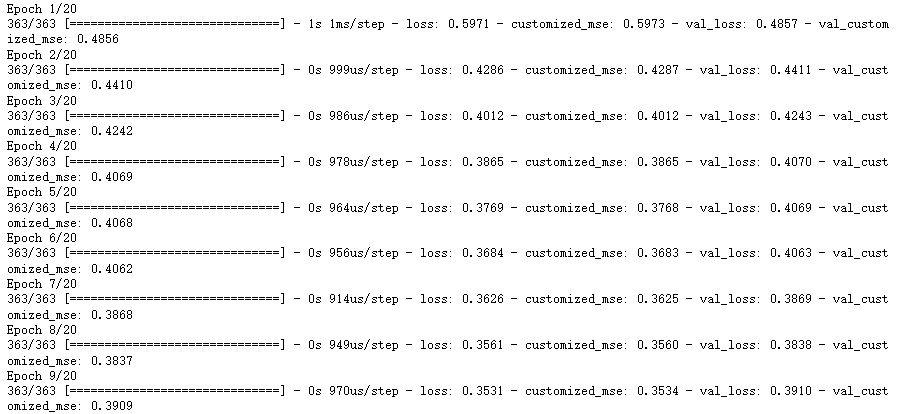


 2967
2967


 被折叠的 条评论
为什么被折叠?
被折叠的 条评论
为什么被折叠?
 到【灌水乐园】发言


