


目录
一、问题描述
二、数据集
三、复习决策树
四、构建决策树
注意:
需要安装的包有:numpy, matplotlib,还有练习自带的代码utils.py。
utils.py没有也没关系,其用途是验证函数编写是否正确,我在代码下方将给出应该运行的结果,与答案一致。代码模块是我自己写的,部分和答案hints不同,但是结果和答案一样,如果有bug请在评论区指出。
源代码将保存在文章底部的链接处。

一、问题描述
假设你正在创办一家种植和销售野生蘑菇的公司。
由于并不是所有的蘑菇都是可食用的,所以您希望能够根据特定蘑菇的物理属性来判断它是可食用的还是有毒的。
您有一些可用于此任务的现有数据。
你能用这些数据来帮助你确定哪些蘑菇可以安全销售吗?
注:所用数据集仅用于说明目的。它并不是用来鉴别食用蘑菇的指南。
二、数据集
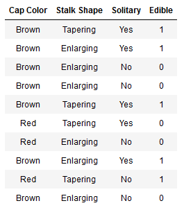
数据集格式如下(表格):
注意:
你有10个样本。每个样本包含三个特征:
蘑菇头的颜色Cap Color(棕色Brown、红色Red)
茎的形状Stalk shape(变大Enlarging、变小Tapering)
独株生长Solitary(是Yes,否No)
一个标签。可食用(1代表可以,0代表不可以)
独热编码
为了方便编写,可以使用独热编码对特征进行改写。
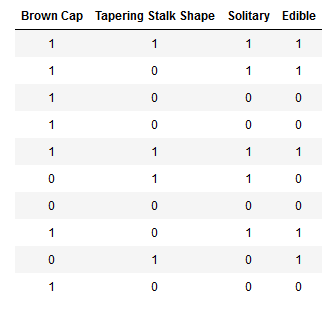
这样,X_train和Y_train变成了只包含0和1的编码。
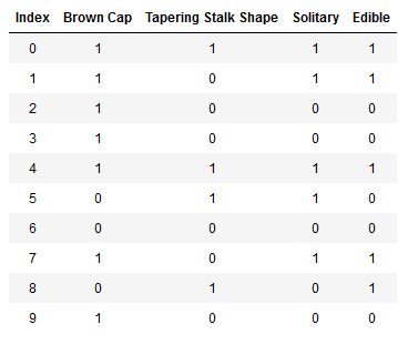
使用独热编码后,X_train和Y_train的表示如下:
X_train = np.array([[1,1,1],[1,0,1],[1,0,0],[1,0,0],[1,1,1],[0,1,1],[0,0,0],[1,0,1],[0,1,0],[1,0,0]])
y_train = np.array([1,1,0,0,1,0,0,1,1,0])
Tips:可以使用np.shape、type(object)详细查看训练集类型和大小。
print ('The shape of X_train is:', X_train.shape)
print ('The shape of y_train is: ', y_train.shape)
print ('Number of training examples (m):', len(X_train))
输出结果:
The shape of X_train is: (10, 3)
The shape of y_train is: (10,)
Number of training examples (m): 10
三、复习决策树
回忆一下决策树的构建过程:
从根节点的所有示例开始
计算所有可能特征的信息增益,并选择信息增益最高的特征
根据所选特征拆分数据集,并创建树的左分支和右分支
继续重复拆分过程,直到满足停止条件
在这一节中,您将实现以下功能,这将允许您使用信息增益最高的功能将节点拆分为左分支和右分支。
计算节点处的熵;
基于给定特征将节点处的数据集拆分为左分支和右分支;
计算在给定特征上拆分的信息增益(Information Gain, IG);
选择使信息增益(Information Gain, IG)最大的特征。
本实验的停止条件为树的深度不超过2
熵的计算
编写compute_entropy函数计算某一结点的熵。
注意:
该函数的输入为标签y,输出为熵。
熵的计算公式如下:

其中,P1表示可食用部分的占比。
为方便计算,设0log2(0) = 0
注意需要检验节点非空。(len(y)!=0)
该部分的代码如下:
# GRADED FUNCTION: compute_entropy
import math
def compute_entropy(y):
    """
    Computes the entropy for

    Args:
       y (ndarray): Numpy array indicating whether each example at a node is
           edible (`1`) or poisonous (`0`)

    Returns:
        entropy (float): Entropy at that node

    """
    # You need to return the following variables correctly
    entropy = 0.

    ### START CODE HERE ###
    if len(y) != 0:
        p_1 = len(y[y == 1]) / len(y)
        if p_1 == 1 or p_1 == 0:
            entropy = 0
        else:
            entropy = -p_1*math.log(p_1,2)-(1-p_1)*math.log(1-p_1,2)
    ### END CODE HERE ###

    return entropy
验证是否正确:
# Since we have 5 edible and 5 non-edible mushrooms, the entropy should be 1"

print("Entropy at root node: ", compute_entropy(y_train))

# UNIT TESTS
compute_entropy_test(compute_entropy
输出结果:
Entropy at root node: 1.0
分割数据集
编写split_dataset函数根据数据集中数据的特征,将其划分入左分支/右分支。
注意:
该函数的输入为:训练数据、该节点的数据点索引列表以及要拆分的特征;
该函数的输出为:左分支/右分支的索引子集。
输入数据格式如下:
约定:可食用(y==1)划入左分支,不可食用(y==0)划入右分支。
代码如下:
# GRADED FUNCTION: split_dataset

def split_dataset(X, node_indices, feature):
    """
    Splits the data at the given node into
    left and right branches

    Args:
        X (ndarray):             Data matrix of shape(n_samples, n_features)
        node_indices (ndarray):  List containing the active indices. I.e, the samples being considered at this step.
        feature (int):           Index of feature to split on

    Returns:
        left_indices (ndarray): Indices with feature value == 1
        right_indices (ndarray): Indices with feature value == 0
    """

    # You need to return the following variables correctly
    left_indices = []
    right_indices = []

    ### START CODE HERE ###
    for i in node_indices:
        if X[i,feature] == 1:
            left_indices.append(i)
        elif X[i,feature] == 0:
            right_indices.append(i)
    ### END CODE HERE ###

    return left_indices, right_indices
验证是否正确:
root_indices = [0, 1, 2, 3, 4, 5, 6, 7, 8, 9]

# Feel free to play around with these variables
# The dataset only has three features, so this value can be 0 (Brown Cap), 1 (Tapering Stalk Shape) or 2 (Solitary)
feature = 0

left_indices, right_indices = split_dataset(X_train, root_indices, feature)

print("Left indices: ", left_indices)
print("Right indices: ", right_indices)

# UNIT TESTS
split_dataset_test(split_dataset)
输出结果:
Left indices: [0, 1, 2, 3, 4, 7, 9]
Right indices: [5, 6, 8]
计算信息增益IG
编写information_gain函数计算信息增益
注意:
该函数的输入为节点处的索引、需要分类的特征、训练样本(X,y),输出为信息增益
信息增益的计算公式如下:

其中,H(P1_node)为根节点的熵;
H(P1_left)为左节点的熵,H(P1_right)为右节点的熵;
w_left为左节点所有样本占全部样本的比例,w_right为右节点所有样本占全部样本的比例。
可以使用compute_entropy()函数计算熵;
可以使用split_dataset()函数分割左右分支。
代码如下:
# GRADED FUNCTION: compute_information_gain

def compute_information_gain(X, y, node_indices, feature):

    """
    Compute the information of splitting the node on a given feature

    Args:
        X (ndarray):            Data matrix of shape(n_samples, n_features)
        y (array like):         list or ndarray with n_samples containing the target variable
        node_indices (ndarray): List containing the active indices. I.e, the samples being considered in this step.

    Returns:
        cost (float):        Cost computed

    """
    # Split dataset
    left_indices, right_indices = split_dataset(X, node_indices, feature)

    # Some useful variables
    X_node, y_node = X[node_indices], y[node_indices]
    X_left, y_left = X[left_indices], y[left_indices]
    X_right, y_right = X[right_indices], y[right_indices]

    # You need to return the following variables correctly
    information_gain = 0

    ### START CODE HERE ###

    # Weights
    w_left = len(X_left) / len(X_node)
    w_right = len(X_right) / len(X_node)
    #Weighted entropy
    H_p1_node = compute_entropy(y)
    H_p1_left = compute_entropy(y_left)
    H_p1_right = compute_entropy(y_right)
    #Information gain
    information_gain = H_p1_node - (w_left*H_p1_left+w_right*H_p1_right)
    ### END CODE HERE ###

    return information_gain
验证结果:
info_gain0 = compute_information_gain(X_train, y_train, root_indices, feature=0)
print("Information Gain from splitting the root on brown cap: ", info_gain0)

info_gain1 = compute_information_gain(X_train, y_train, root_indices, feature=1)
print("Information Gain from splitting the root on tapering stalk shape: ", info_gain1)

info_gain2 = compute_information_gain(X_train, y_train, root_indices, feature=2)
print("Information Gain from splitting the root on solitary: ", info_gain2)

# UNIT TESTS
compute_information_gain_test(compute_information_gain)
输出结果:
Information Gain from splitting the root on brown cap: 0.034851554559677034
Information Gain from splitting the root on tapering stalk shape: 0.12451124978365313
Information Gain from splitting the root on solitary: 0.2780719051126377
(结果表明独株生长Solitary,features=2的信息增益最大,最适合作为根节点向下分裂的特征)
得到最佳分支
编写get_best_split()函数,根据上面得到的信息增益,获取对应的特征。
注意:
该函数接收训练样本及其索引,返回最佳特征。
可以使用compute_information_gain()函数帮助你计算信息增益。
代码如下:
# GRADED FUNCTION: get_best_split

def get_best_split(X, y, node_indices):
    """
    Returns the optimal feature and threshold value
    to split the node data

    Args:
        X (ndarray):            Data matrix of shape(n_samples, n_features)
        y (array like):         list or ndarray with n_samples containing the target variable
        node_indices (ndarray): List containing the active indices. I.e, the samples being considered in this step.

    Returns:
        best_feature (int):     The index of the best feature to split
    """

    # Some useful variables
    num_features = X.shape[1]

    # You need to return the following variables correctly
    best_feature = -1

    ### START CODE HERE ###
    IG = []
    for i in range(num_features):
        IG.append(compute_information_gain(X, y, node_indices, i))
    best_feature = np.argmax(IG)
    ### END CODE HERE ##

    return best_feature
验证结果:
best_feature = get_best_split(X_train, y_train, root_indices)
print("Best feature to split on: %d" % best_feature)

# UNIT TESTS
get_best_split_test(get_best_split)
输出结果:
Best feature to split on: 2
四、构建决策树
代码如下:
def build_tree_recursive(X, y, node_indices, branch_name, max_depth, current_depth):
    """
    Build a tree using the recursive algorithm that split the dataset into 2 subgroups at each node.
    This function just prints the tree.

    Args:
        X (ndarray):            Data matrix of shape(n_samples, n_features)
        y (array like):         list or ndarray with n_samples containing the target variable
        node_indices (ndarray): List containing the active indices. I.e, the samples being considered in this step.
        branch_name (string):   Name of the branch. ['Root', 'Left', 'Right']
        max_depth (int):        Max depth of the resulting tree.
        current_depth (int):    Current depth. Parameter used during recursive call.

    """

    # Maximum depth reached - stop splitting
    if current_depth == max_depth:
        formatting = " "*current_depth + "-"*current_depth
        print(formatting, "%s leaf node with indices" % branch_name, node_indices)
        return

    # Otherwise, get best split and split the data
    # Get the best feature and threshold at this node
    best_feature = get_best_split(X, y, node_indices)
    tree.append((current_depth, branch_name, best_feature, node_indices))

    formatting = "-"*current_depth
    print("%s Depth %d, %s: Split on feature: %d" % (formatting, current_depth, branch_name, best_feature))

    # Split the dataset at the best feature
    left_indices, right_indices = split_dataset(X, node_indices, best_feature)

    # continue splitting the left and the right child. Increment current depth
    build_tree_recursive(X, y, left_indices, "Left", max_depth, current_depth+1)
    build_tree_recursive(X, y, right_indices, "Right", max_depth, current_depth+1)
验证结果:
build_tree_recursive(X_train, y_train, root_indices, "Root", max_depth=2, current_depth=0)输出结果:
Depth 0, Root: Split on feature: 2
- Depth 1, Left: Split on feature: 0
-- Left leaf node with indices [0, 1, 4, 7]
-- Right leaf node with indices [5]
- Depth 1, Right: Split on feature: 1
-- Left leaf node with indices [8]
-- Right leaf node with indices [2, 3, 6, 9]
小结
决策树主要的函数包括:熵的计算compute_entropy(),分割数据集(左右分支)split_dataset(),计算信息增益information_gain(),得到最佳分支节点get_best_split(),构建决策树build_tree_recursive()。
源代码链接:
夸克网盘


 6132
6132

 被折叠的 条评论
为什么被折叠?
被折叠的 条评论
为什么被折叠?
 到【灌水乐园】发言


