Machine Learning Project 2 Part A

Machine Learning Project 2 Part A

Support vector machines
This Tropic Project is the project of ESIEE Paris’Machine Learning course, TP by Prof. Hilaire xavier.
This TP was finished by WANG zihao

• April 13, 2015
• Inspecting data
• Common work
• Strategy A : Bayes classi cation
• Strategy B : SVM and decision trees

Contents

Inspecting data

Open MPEG-7/index.html in a browser, and inspect the images there. Beware that the images appearing are only previews of real images, and these previews are normalized to have a height of 100 pixels. In general, samples belonging to a given class are neither rescaled, nor recentered; they may also appear as rotated versions of the object they represent.

图像特征提取（Features Extraction）

HU-不变矩方法

Hu在其《Visual Pattern Recognition by Moment Invariants》1首次提出了不变矩方法来对图像进行特征提取。

可以看出，不变矩作用主要目的是描述事物（图像）的特征。人眼识别图像的特征往往又表现为“求和”的形式，因此不变矩是对图像元素进行了积分操作。
不变矩能够描述图像整体特征就是因为它具有平移不变形、比例不变性和旋转不变性等性质。2
To summarize and make the image samples independent of translation, scale, and rotation, we might think of the Hu moments as putative features. The Hu moments are the I1 : I7 expressions summarized here:3. The original paper from Hu can be found in the Papers directory, along with one of Flusser { who not only provides a much simpler derivation using complex roots, but also showed that original Hu basis formed by the 7 invariants was incomplete, as an 8th invariant does exist.
The cent moment.m and feature vec.m les compute the 7 Hu moments given an input pat-tern. The hu image.m le does the same, but from an image whose countours are extracted using simple morphological operations.

Hu-Method

function [ f ] = hu_image(A)
    % compute the contour using simple morpho. math
    cont=A-imerode(A,strel('disk',1));
    cont=double(cont > 0);  % make it binary

    figure, imshow(cont);
    f=feature_vec(cont);
end

%Extract Hu-moment of two different classes one is the pic of bat, theother is thhe pic of dog.
% Code by WANG zihao 2015-04-21
clear all 
clc
close all

A = hu_moments('MPEG-7/apple-1*gif');
B = hu_moments('MPEG-7/bat-1*gif');

close all

A = A(1:9,:)
B = B(1:9,:)

%%%savefileA = 'mat1.m'
%%%savefileB = 'mat2.m'
%%%save(savefileA,'A')
%%%save(savefileB,'B')



savefileA = 'mat1.mat';
savefileB = 'mat2.mat';
save mat1 A
save mat2 B



keyboard
figure(1)

x = A(:,1)
y = A(:,2)
z = A(:,3)
subplot(321)
scatter3(x,y,z,'b')
hold on
x = B(:,1)
y = B(:,2)
z = B(:,3)
scatter3(x,y,z,'r','filled')
title('1-3');


x = A(:,2)
y = A(:,3)
z = A(:,4)
subplot(322)
scatter3(x,y,z,'b')
hold on
x = B(:,2)
y = B(:,3)
z = B(:,4)
scatter3(x,y,z,'r','filled')
title('2-4')

x = A(:,3)
y = A(:,4)
z = A(:,5)
subplot(323)
scatter3(x,y,z,'b')
hold on
x = B(:,3)
y = B(:,4)
z = B(:,5)
scatter3(x,y,z,'r','filled')
title('3-5')

x = A(:,4)
y = A(:,5)
z = A(:,6)
subplot(324)
scatter3(x,y,z,'b')
hold on
x = B(:,4)
y = B(:,5)
z = B(:,6)
scatter3(x,y,z,'r','filled')
title('4-6')


x = A(:,5)
y = A(:,6)
z = A(:,7)
subplot(325)
scatter3(x,y,z,'b')
hold on

x = B(:,5)
y = B(:,6)
z = B(:,7)
scatter3(x,y,z,'r','filled')
title('6-7')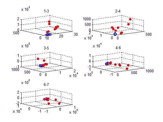 

Common Work

Question 4

Evolution of the models ,return the best model.

Both strategies below approximate the problem of multiclass classi cation, using only 2-class SVMs. You will need a procedure [R] = autosvm(C1,C2) that will automatically return the best C-SVM classi cator for classes C1 and C2 (whose size might be very dierent), considering serveral values of C and kernel parameters.
Write this function, using either the fitcsvm function from Matlab’s ML Toolbox and let Matlab adjust parameters for training, or write code of your own based on that written for TD3, and directly control the C constant and kernel parameters. The return value can be either the Matlab SVMModel stucture, or a strtucture of your own.
Try linear, RBF (gaussian) and polynomial kernels. But remember that when attempting to separate 2 vanilla classes, you might be working with as low as 20 samples per class. So do not push degrees to far, or it will result in serious over ting issues very quickly. Balance between training/testing data should typically be at least 70%=30%. Depending on the classes you have chosen, you might also come to use 1 testing pattern against n-1 training pattern, and average the solutions in the dual space.

Matlab Functions

Note, If you use a MATLAB before version R2014 you should use the function

                        svmtrain()

Load Fisher’s iris data set. Remove the sepal lengths and widths, and all observed setosa irises.

                SVMModel = fitcsvm(X,y)

SVMModel = fitcsvm(X,Y) returns a support vector machine classifier SVMModel, trained by predictors X and class labels Y for one- or two-class classification.

load fisheriris
inds = ~strcmp(species,'setosa');
X = meas(inds,3:4);
y = species(inds);
Train an SVM classifier using the processed data set.
%Called below
SVMModel = fitcsvm(X,y)

[Matlab SVM] http://fr.mathworks.com/help/stats/fitcsvm.html

DATA STRUCTURE OF TWO DIFFERENT CLASSES　
Class A Bats pictures

Class A Bats	Fatures 1	Fatures 2	Fatures 3	Fatures 4	Fatures 5	Fatures 6	Fatures 7
Picture 1
Picture 2
Picture 3
Picture 4
Picture 5
Picture 6
Picture 7
Picture 8
Picture 9

Class B Dogs Pictures

Class B Dogs	Fatures 1	Fatures 2	Fatures 3	Fatures 4	Fatures 5	Fatures 6	Fatures 7
Picture 1
Picture 2
Picture 3
Picture 4
Picture 5
Picture 6
Picture 7
Picture 8
Picture 9

M file

%The Question 4 of COMMON WORK, because of the our matlab is 2013 %we use The svmtrain() function to replace fitcsvm()
%Job done by Zihao WANG 2015-04-21
%C1 and C2 are two classes from .mat file 
function [R] = autosvm(C1,C2,ratio)
A = C1;
B = C2;
%Class_A is the Class of BATs
Class_A = 0;
%Class_A is the Class of DOGs
Class_B = 1;
[m n] = size(A);
r = ratio;%THE NUMBER OF TRANING DATA
traning = [A(1:r,:); B(1:r,:)];
testing = [A(r+1:m,:); B(r+1:m,:)];

Group = zeros(2*r,1);
Group(1:r) = Class_A;
Group(r+1:2*r) = Class_B;
Group = Group';
Group_A_T = zeros((m-r),1)
Group_B_T = zeros((m-r),1)+1
Group_test = [Group_A_T;Group_B_T];
SVMStruct = svmtrain(traning, Group);

C = svmclassify(SVMStruct,testing);
R = C;
errRate = sum(Group_test~= C)/2  %mis-classification rate
conMat = confusionmat(Group_test,C) % the confusion matrix

running result

errRate =

 0

conMat =

 5     0
 0     5

Linkedin ：http://www.linkedin.com/profile/view?id=307187546
Email : zihao.wang@edu.esiee.fr
Weibo： http://weibo.com/mrzihaowang/
Facebook：http://www.facebook.com/zinhoowong
twitter: https://twitter.com/WongZinhoo