


任务描述-域自适应
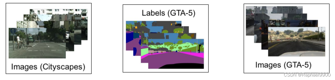
●想象一下,你想做与3D环境相关的任务,然后发现
○3D图像很难标记,因此也很昂贵。
○模拟图像(如GTA-5上的模拟场景)很容易标记。为什么不仅仅对模拟图像进行训练呢?
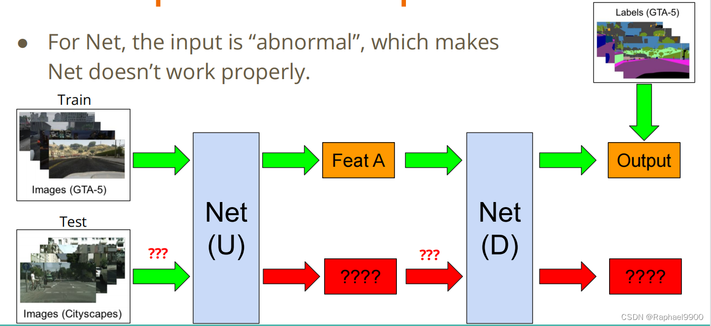
●对于Net,输入是“异常的”的,这使得Net不能正常工作。
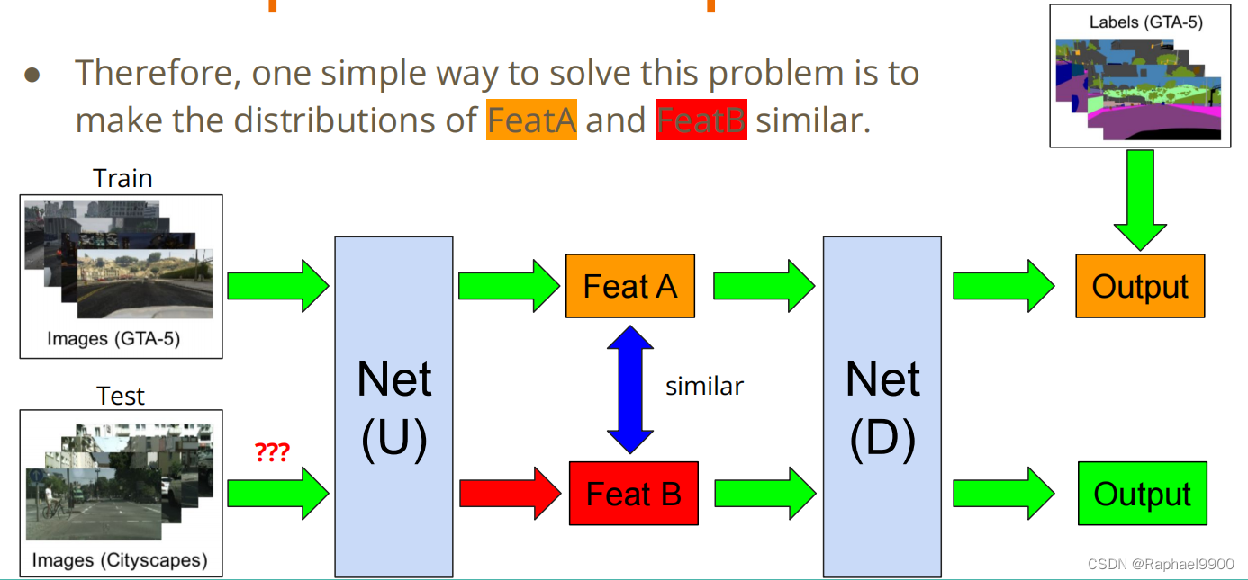
●因此,解决这个问题的一个简单方法是使FeatA和FeatB的分布相似。
 ●我们的任务:给定真实的图像(带标签)和绘图图像(无标签),请使用域自适应技术,使您的网络正确地预测绘图图像。
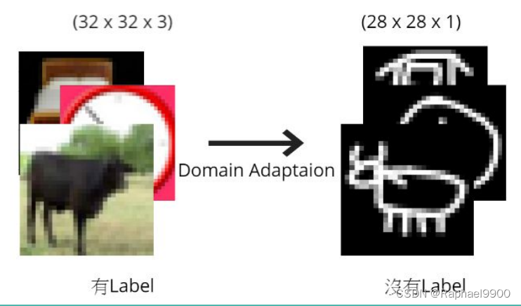
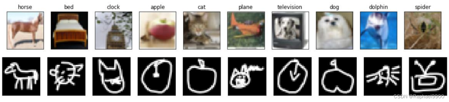
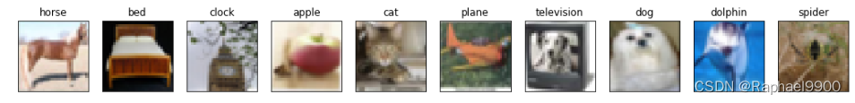
●标签: 10个类(编号从0到9),如下图片所示。
●训练: 5000(32、32)RGB真实图像(带有标签)。
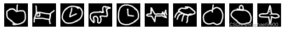
●测试: 100000(28,28)灰度绘图图像。
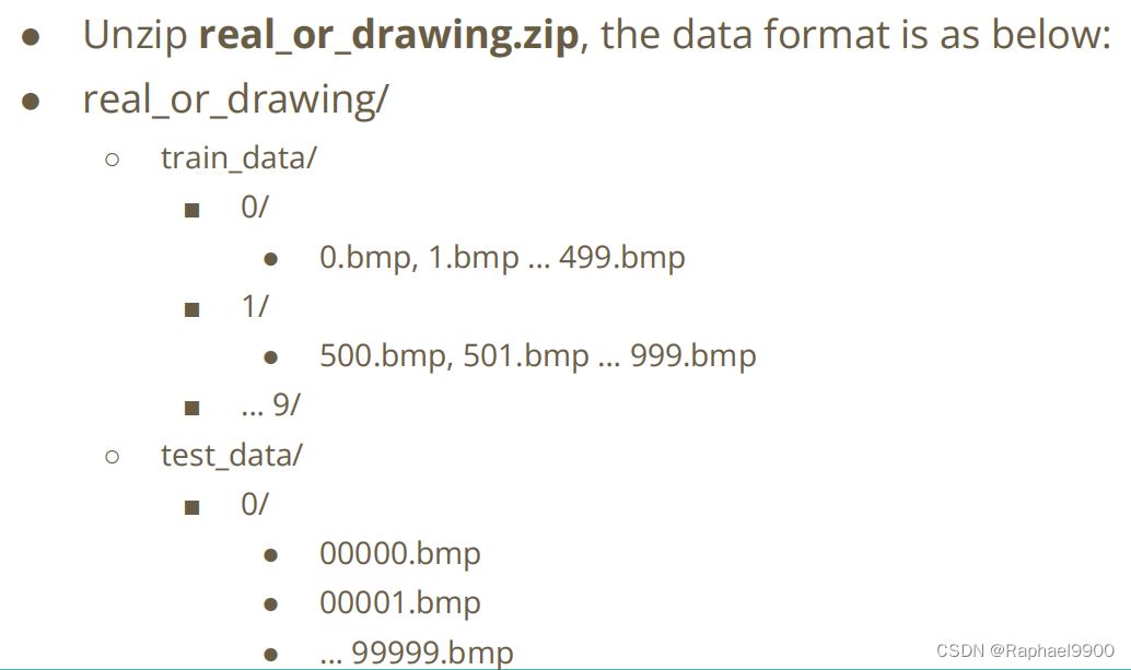
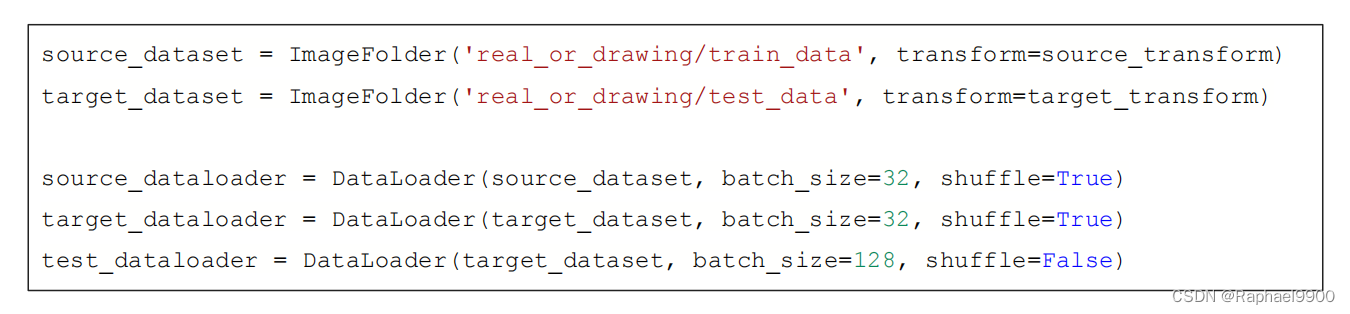
●您可以简单地使用以下代码来获取数据处理器。(您可以应用您自己的源/目标变换函数。)
二、代码
场景和为什么进行领域对抗培训?
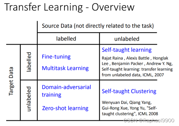
现在我们已经标记了源数据和未标记的目标数据,其中源数据可能与目标数据相关。我们现在希望仅使用源数据训练模型,并在目标数据上测试它。
如果我们这样做,会出现什么问题?在我们学习了异常检测之后,我们现在知道,如果我们用从未出现在源数据中的异常数据来测试模型,我们训练的模型很可能会导致较差的性能,因为它不熟悉异常数据。
例如,我们有一个包含特征提取器和分类器的模型:
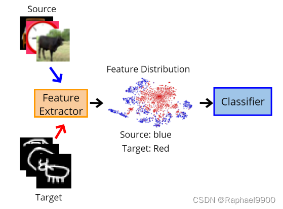
当用源数据训练模型时,特征提取器将提取有意义的特征,因为它熟悉源数据的分布。从下图中可以看出,蓝点(源数据的分布)已经被聚类到不同的簇中。因此,分类器可以基于这些聚类来预测标签。
然而,当在目标数据上测试时,特征提取器将不能提取遵循源特征分布的有意义的特征,这导致为源领域学习的分类器将不能应用于目标领域。
神经网络的领域对抗训练
基于上述问题,DaNN方法在源(训练时)域和目标(测试时)域之间建立映射,使得为源域学习的分类器在与域之间的学习映射组合时也可以应用于目标域。
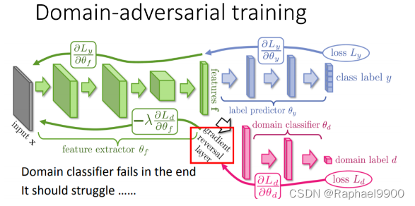
在DaNN中,作者在训练框架中增加了一个领域分类器,它是一个经过深度区分训练的分类器,通过特征提取器提取的特征来区分来自不同领域的数据。随着训练的进行,该方法促进了区分源域和目标域的域分类器,以及能够提取特征的特征提取器,该特征对于源域上的主要学习任务是有区别的,并且对于域之间的转移是无差别的。
特征提取器可能优于领域分类器,因为其输入是由特征提取器生成的,并且领域分类和标签分类的任务不冲突。
这种方法导致出现领域不变的特征,并且在相同的特征分布上。
我们的任务包含源数据:真实照片,目标数据:手绘涂鸦。我们要用照片和标签训练模型,试着预测手绘涂鸦的标签是什么。
import matplotlib.pyplot as plt

def no_axis_show(img, title='', cmap=None):
  # imshow, and set the interpolation mode to be "nearest"。
  fig = plt.imshow(img, interpolation='nearest', cmap=cmap)
  # 不要在图像中显示轴。
  fig.axes.get_xaxis().set_visible(False)
  fig.axes.get_yaxis().set_visible(False)
  plt.title(title)

# 显示训练数据的十个图片
titles = ['horse', 'bed', 'clock', 'apple', 'cat', 'plane', 'television', 'dog', 'dolphin', 'spider']
plt.figure(figsize=(18, 18))
for i in range(10):
  plt.subplot(1, 10, i+1)
  fig = no_axis_show(plt.imread(f'real_or_drawing/train_data/{i}/{500*i}.bmp'), title=titles[i])
#读取测试数据的十个图片
plt.figure(figsize=(18, 18))
for i in range(10):
  plt.subplot(1, 10, i+1)
  fig = no_axis_show(plt.imread(f'real_or_drawing/test_data/0/' + str(i).rjust(5, '0') + '.bmp'))
特殊领域知识
当我们涂鸦时,我们通常只画轮廓,因此我们可以对源数据进行边缘检测处理,使其与目标数据更加相似。
Canny边缘检测
Canny边缘检测实现如下。
用CV2实现Canny边缘检测只需要两个参数:low_threshold和high_threshold。
cv2.Canny(image, low_threshold, high_threshold)
简单来说,当边缘值超过high_threshold时,我们将其确定为边缘。如果边缘值仅高于low_threshold,那么我们将确定它是否是边缘。让我们在源数据上实现它。
import cv2
import matplotlib.pyplot as plt
titles = ['horse', 'bed', 'clock', 'apple', 'cat', 'plane', 'television', 'dog', 'dolphin', 'spider']
plt.figure(figsize=(18, 18))

original_img = plt.imread(f'real_or_drawing/train_data/0/0.bmp')#图片读取
plt.subplot(1, 5, 1)#将多个图画到一个平面上
no_axis_show(original_img, title='original')

gray_img = cv2.cvtColor(original_img, cv2.COLOR_RGB2GRAY)
plt.subplot(1, 5, 2)
no_axis_show(gray_img, title='gray scale', cmap='gray')

canny_50100 = cv2.Canny(gray_img, 50, 100)#边缘检测算法
plt.subplot(1, 5, 3)
no_axis_show(canny_50100, title='Canny(50, 100)', cmap='gray')

canny_150200 = cv2.Canny(gray_img, 150, 200)
plt.subplot(1, 5, 4)
no_axis_show(canny_150200, title='Canny(150, 200)', cmap='gray')

canny_250300 = cv2.Canny(gray_img, 250, 300)
plt.subplot(1, 5, 5)
no_axis_show(canny_250300, title='Canny(250, 300)', cmap='gray')

这些数据适用于torchvision.ImageFolder。
import numpy as np
import torch
import torch.nn as nn
import torch.nn.functional as F
from torch.autograd import Function

import torch.optim as optim
import torchvision.transforms as transforms
from torchvision.datasets import ImageFolder
from torch.utils.data import DataLoader

source_transform = transforms.Compose([
    # 将RGB转换为灰度。(因为Canny不支持RGB图像。)
    transforms.Grayscale(),
    # cv2不支持skimage.image,所以我们把它转换成np.array,
    # 然后采用cv2.Canny算法。
    transforms.Lambda(lambda x: cv2.Canny(np.array(x), 170, 300)),
    # Transform np.array back to the skimage.Image.
    transforms.ToPILImage(),
    #50%水平翻转。(用于增强)
    transforms.RandomHorizontalFlip(),
#旋转+- 15度。(用于增强),并用零填充
#如果旋转后有空像素。
    transforms.RandomRotation(15, fill=(0,)),
    # 转换为模型输入的张量。
    transforms.ToTensor(),
])
target_transform = transforms.Compose([
    # Turn RGB to grayscale.
    transforms.Grayscale(),
    #调整大小:源数据的大小是32x32,因此我们需要
#将目标数据得大小从28x28放大到32x32 .
    transforms.Resize((32, 32)),
    # 50% Horizontal Flip. (For Augmentation)
    transforms.RandomHorizontalFlip(),
    # Rotate +- 15 degrees. (For Augmentation), and filled with zero
    # if there's empty pixel after rotation.
    transforms.RandomRotation(15, fill=(0,)),
    # Transform to tensor for model inputs.
    transforms.ToTensor(),
])

source_dataset = ImageFolder('real_or_drawing/train_data', transform=source_transform)
target_dataset = ImageFolder('real_or_drawing/test_data', transform=target_transform)

source_dataloader = DataLoader(source_dataset, batch_size=32, shuffle=True)
target_dataloader = DataLoader(target_dataset, batch_size=32, shuffle=True)
test_dataloader = DataLoader(target_dataset, batch_size=128, shuffle=False)
特征提取器:经典的VGG式结构
标签预测器/域分类器:线性模型。
class FeatureExtractor(nn.Module):

    def __init__(self):
        super(FeatureExtractor, self).__init__()

        self.conv = nn.Sequential(
            nn.Conv2d(1, 64, 3, 1, 1),
            nn.BatchNorm2d(64),
            nn.ReLU(),
            nn.MaxPool2d(2),

            nn.Conv2d(64, 128, 3, 1, 1),
            nn.BatchNorm2d(128),
            nn.ReLU(),
            nn.MaxPool2d(2),

            nn.Conv2d(128, 256, 3, 1, 1),
            nn.BatchNorm2d(256),
            nn.ReLU(),
            nn.MaxPool2d(2),

            nn.Conv2d(256, 256, 3, 1, 1),
            nn.BatchNorm2d(256),
            nn.ReLU(),
            nn.MaxPool2d(2),

            nn.Conv2d(256, 512, 3, 1, 1),
            nn.BatchNorm2d(512),
            nn.ReLU(),
            nn.MaxPool2d(2)
        )

    def forward(self, x):
        x = self.conv(x).squeeze()
        return x

class LabelPredictor(nn.Module):

    def __init__(self):
        super(LabelPredictor, self).__init__()

        self.layer = nn.Sequential(
            nn.Linear(512, 512),
            nn.ReLU(),

            nn.Linear(512, 512),
            nn.ReLU(),

            nn.Linear(512, 10),
        )

    def forward(self, h):
        c = self.layer(h)
        return c

class DomainClassifier(nn.Module):

    def __init__(self):
        super(DomainClassifier, self).__init__()

        self.layer = nn.Sequential(
            nn.Linear(512, 512),
            nn.BatchNorm1d(512),
            nn.ReLU(),

            nn.Linear(512, 512),
            nn.BatchNorm1d(512),
            nn.ReLU(),

            nn.Linear(512, 512),
            nn.BatchNorm1d(512),
            nn.ReLU(),

            nn.Linear(512, 512),
            nn.BatchNorm1d(512),
            nn.ReLU(),

            nn.Linear(512, 1),
        )

    def forward(self, h):
        y = self.layer(h)
        return y
预训练:这里我们使用Adam作为我们的优化器。
feature_extractor = FeatureExtractor().cuda()
label_predictor = LabelPredictor().cuda()
domain_classifier = DomainClassifier().cuda()

class_criterion = nn.CrossEntropyLoss()
domain_criterion = nn.BCEWithLogitsLoss()

optimizer_F = optim.Adam(feature_extractor.parameters())
optimizer_C = optim.Adam(label_predictor.parameters())
optimizer_D = optim.Adam(domain_classifier.parameters())
DaNN实现
在原始论文中,使用了梯度反转层Gradient Reversal Layer。特征提取器、标签预测器和领域分类器都同时被训练。在这段代码中,我们首先训练领域分类器,然后训练我们的特征提取器(与GAN中的生成器和鉴别器训练过程的概念相同)。
控制领域对抗损失的λ在原始论文中是自适应的。simple的λ设置为0.1。没有目标数据的标签。
def train_epoch(source_dataloader, target_dataloader, lamb):
'''
Args:
source_dataloader: source data的dataloader
target_dataloader: target data的dataloader
lamb: control the balance of domain adaptatoin and classification.
'''
# D loss: Domain Classifier的loss
# F loss: Feature Extrator & Label Predictor的loss
running_D_loss, running_F_loss = 0.0, 0.0
total_hit, total_num = 0.0, 0.0
for i, ((source_data, source_label), (target_data, _)) in enumerate(zip(source_dataloader, target_dataloader)):
source_data = source_data.cuda()
source_label = source_label.cuda()
target_data = target_data.cuda()
#混合源数据和目标数据,否则会误导batch_norm的运行参数
# (runnning mean/var of soucre and target data are different.)
mixed_data = torch.cat([source_data, target_data], dim=0)
domain_label = torch.zeros([source_data.shape[0] + target_data.shape[0], 1]).cuda()#目标数据的标签设置为0
#将源数据的域标签设置为1,
domain_label[:source_data.shape[0]] = 1
# Step 1 : train domain classifier
feature = feature_extractor(mixed_data)
#我们不需要在步骤1中训练特征提取器。
#因此,我们分离特征神经元以避免反向传播。
domain_logits = domain_classifier(feature.detach())
loss = domain_criterion(domain_logits, domain_label)
running_D_loss+= loss.item()
loss.backward()
optimizer_D.step()
# Step 2 : train feature extractor and label classifier
class_logits = label_predictor(feature[:source_data.shape[0]])
domain_logits = domain_classifier(feature)
# loss = cross entropy of classification - lamb * domain binary cross entropy.
# 在GAN判别器中使用减法类似于generator loss的原因
loss = class_criterion(class_logits, source_label) - lamb * domain_criterion(domain_logits, domain_label)
running_F_loss+= loss.item()
loss.backward()
optimizer_F.step()
optimizer_C.step()
optimizer_D.zero_grad()
optimizer_F.zero_grad()
optimizer_C.zero_grad()
total_hit += torch.sum(torch.argmax(class_logits, dim=1) == source_label).item()
total_num += source_data.shape[0]
print(i, end='\r')
return running_D_loss / (i+1), running_F_loss / (i+1), total_hit / total_num
print('start training')
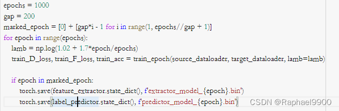
epochs = 1000
gap = 200
marked_epoch = [0] + [gap*i - 1 for i in range(1, epochs//gap + 1)]
for epoch in range(epochs):
lamb = np.log(1.02 + 1.7*epoch/epochs)
train_D_loss, train_F_loss, train_acc = train_epoch(source_dataloader, target_dataloader, lamb=lamb)
if epoch in marked_epoch:
torch.save(feature_extractor.state_dict(), f'extractor_model_{epoch}.bin')
torch.save(label_predictor.state_dict(), f'predictor_model_{epoch}.bin')
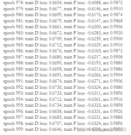
print('epoch {:>3d}: train D loss: {:6.4f}, train F loss: {:6.4f}, acc {:6.4f}'.format(epoch, train_D_loss, train_F_loss, train_acc))
torch.save(feature_extractor.state_dict(), f'extractor_model.bin')
torch.save(label_predictor.state_dict(), f'predictor_model.bin')
我们使用pandas来生成我们的csv文件。经过200 epoches的模型的性能可能不稳定,可以训练更多的epoches,以获得更稳定的性能。
result = []
label_predictor.eval()
feature_extractor.eval()
for i, (test_data, _) in enumerate(test_dataloader):
test_data = test_data.cuda()
class_logits = label_predictor(feature_extractor(test_data))
x = torch.argmax(class_logits, dim=1).cpu().detach().numpy()
result.append(x)
import pandas as pd
result = np.concatenate(result)#numpy中对array进行拼接的函数
# Generate your submission
df = pd.DataFrame({'id': np.arange(0,len(result)), 'label': result})
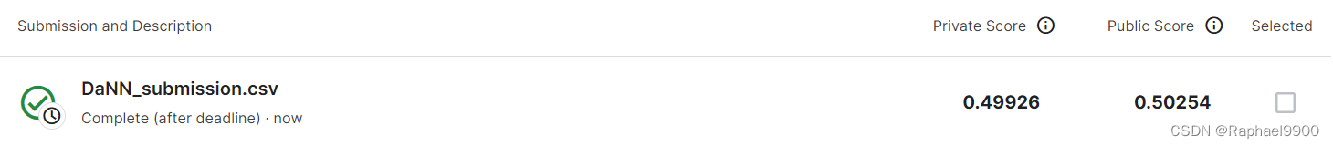
df.to_csv('DaNN_submission.csv',index=False)
三、实验
1、Simple Baseline
直接运行助教代码。
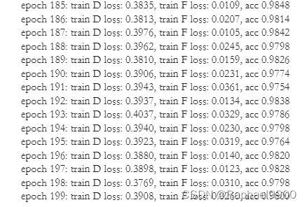
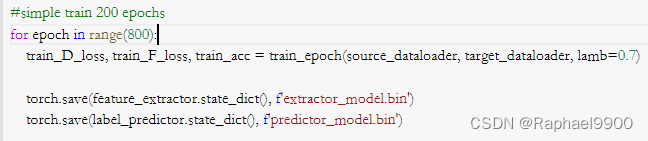
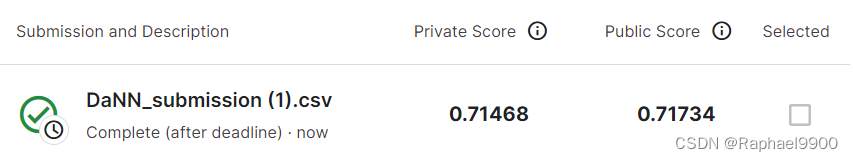
2、Medium Baseline
方法:增加epoch+ 改变lamb。epoch从200增加到800,lamb从0.1变为0.7。提升lamb意味着更注重domain classifier的表现,让source domain和target domain的表现更一致。不过也不能一直提升,会影响label predictor的能力。
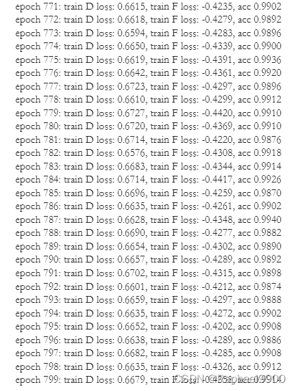
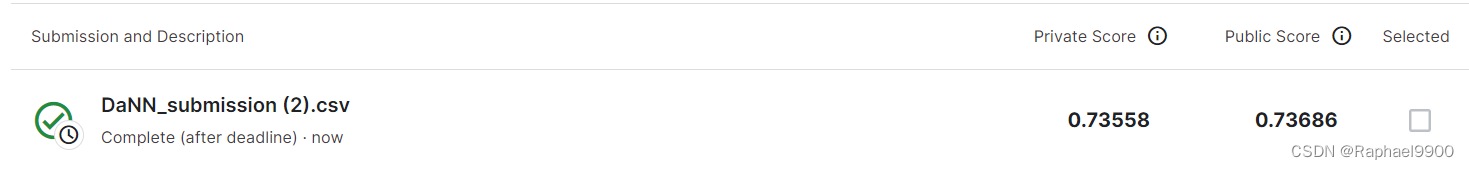
3、Strong Baseline
方法:增加epoch+ 动态调整lamb值。将epoch调整到1000。可使用动态调整的lamb值,从0.02动态的调整为1,这样前期可让labelpredictor更准确,后期更注重domainclassifier的表现。


 8164
8164


 被折叠的 条评论
为什么被折叠?
被折叠的 条评论
为什么被折叠?
 到【灌水乐园】发言


