多项式曲线拟合MATLABcensus.mat数据

多项式曲线拟合

0.题目背景

针对MATLAB提供的census.mat数据，用多项式拟合方法进行曲线拟合，确定其数学模型，并给出拟合过程及分析。

1. 相关性分析

• 原理

  • 协方差矩阵

    • $corrcoef(X,Y)=\left[\begin{array}{cc}Cov(X,X)& Cov(X,Y)\\ Cov(Y,X)& Cov(Y,Y)\end{array}\right]$
    • 数字越接近于1 说明相关性越强

• 分析过程及部分代码

  • 散点图绘制

  plot(cdate,pop,'om')  
  title('U.S. Population from 1790 to 1990');  
  xlabel('Census Year');  
  ylabel('Population (millions)');  
  

  

  • 计算协方差矩阵

  >> corrcoef(cdate,pop)
    
      ans =
  
        1.0000    0.9597
        0.9597    1.0000
  

• 结论

  1. 从图像上可以直观地看出原始样本数据具有较强的相关性
  2. 协方差矩阵系数都接近于1,进一步证明数据的强相关性

2. 多项式拟合

• 原理

  • Feature scaling(特征缩放)–Standardization(标准化)

    • 对不同特征维度的伸缩变换的目的是使得不同度量之间的特征具有可比性,对目标函数的影响体现在**几何分布上，同时不改变原始数据的分布。**

    • 特征标准化使数据中每个特征的值具有零均值（当减去分子中的均值时）和单位方差。该方法广泛用于许多机器学习算法（例如，支持向量机、逻辑回归和人工神经网络）中的归一化。

      ​ $X^{\ast }=\frac{X-\bar{X}}{\sigma }$

    • (cdate-mean(cdate))./std(cdate); 
      //代码演示
      

    • 工具箱内勾选"Center and Scale"

  • 通过Curve Fitting Tool工具箱绘制拟合图像和残差图

• 部分代码和图像

  • 初始化数据

  • %% Initialization.
    
    % Initialize arrays to store fits and goodness-of-fit.
    fitresult = cell( 2, 1 );
    gof = struct( 'sse', cell( 2, 1 ), ...
      'rsquare', [], 'dfe', [], 'adjrsquare', [], 'rmse', [] );
    
    

  • 拟合曲线(注:这里只贴出poly2的源码)

    %% Fit: 'poly2'.
    [xData, yData] = prepareCurveData( cdate, pop );
    
    % Set up fittype and options.
    ft = fittype( 'poly2' );
    
    % Fit model to data.
    [fitresult{1}, gof(1)] = fit( xData, yData, ft, 'Normalize', 'on' );
    
    % Create a figure for the plots.
    figure( 'Name', 'poly2' );
    
    % Plot fit with data. 
    subplot( 2, 1, 1 );
    h = plot( fitresult{1}, xData, yData );
    legend( h, 'pop vs. cdate', 'poly2', 'Location', 'NorthEast' );
    % Label axes
    xlabel cdate
    ylabel pop
    grid on
    
    % Plot residuals.
    subplot( 2, 1, 2 );
    h = plot( fitresult{1}, xData, yData, 'residuals' );
    legend( h, 'poly2 - residuals', 'Zero Line', 'Location', 'NorthEast' );
    
    % Label axes
    xlabel cdate
    ylabel pop
    grid on
    

  • poly2~poly6,exp2的拟合曲线及残差图

3. 拟合优度分析

• 原理

  1. SSE(残差平方和): the Sum of Square due to Error

     $SSres={\sum }_{i=1}^n(y_i-\hat{y}{)}^2=e_i^2$

     该参数越接近于0,表示曲线拟合越成功

  2. RMSE(均方根误差、标准差)：Root mean squared error

     $RMSE=\sqrt{MSE}=\sqrt{\frac{SSE}{n}}=\sqrt{\frac{1}{n}{\sum }_{i=1}^n(y_i-\overline{y_i}{)}^2}$

     每个误差对 RMSE 的影响与平方误差的大小成正比；因此较大的误差对 RMSE 的影响非常大,所以RMSE 对异常值很敏感。

  MSE(均方差、方差)：Mean squared error

  数理统计中均方误差是指参数估计值与参数值之差平方的期望值，记为MSE。MSE是衡量**“平均误差”**的一种较方便的方法，**MSE可以评价数据的变化程度，MSE的值越小，说明预测模型描述实验数据具有更好的精确度。**预测数据和原始数据对应点误差平方和的均值

  $MSE=\frac{SSE}{n}$

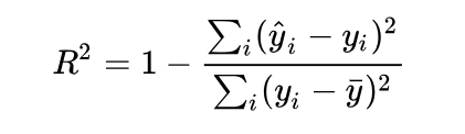
  3. R-square($R^2$)(决定系数):Coefficient of determination

     ​ R² 即判定系数，也称为拟合优度 // **区分于相关系数r和$\rho xy$**​

     ​ 拟合优度越大，自变量对因变量的解释程度越高，自变量引起的变动占总变动的百分比就越高。观察点在回归直线附近越密集。取值范围：0-1.

  ​ $R_2=1-\frac{SSres}{SStot}$
  

  $SSreg={\sum }_{i=1}^n(\hat{y}-\bar{y}{)}^2$

  $SSres={\sum }_{i=1}^n(y_i-\hat{y}{)}^2=e_i^2$

  $SStot={\sum }_{i=1}^n(y_i-\bar{y}{)}^2$

  回归平方和：SSR(Sum of Squares for regression) = ESS (explained sum of squares)

  残差平方和：SSE(Sum of Squares for Error） = RSS(residual sum of squares)

  总离差平方和：SST(Sum of Squares for total) = TSS(total sum of squares)

  **SSE+SSR=SST **

  RSS+ESS=TSS

  4. $R^2_adj $ (校正决定系数): adjust R-square

     ​ R² 评价拟合模型的好坏具有一定的局限性，即使向模型中增加的变量没有统计学意义，R²值仍会增大。因此需对其进行校正，从而形成了校正的决定系数(Adj R²) 。与R² 不同的是，当模型中增加的变量没有统计学意义时，Adj R²会减小，因此Adj R² 是衡量所建模型好坏的重要指标之一，Adj R^2 越大，模型拟合得越好。

  校正决定系数（Adj R²）引入了样本数量和特征数量，公式如下：

  ​ $R^{2}adj=1-\frac{(1-R^2)(n-1)}{n-p-1}$

• 分析过程及部分代码

  • 拟合人口普查数据的目的是预测出未来人口数

    • 对于poly6来说,数据明显超出了我们想要得到的结果,因此ploy6舍去
    • 
    • 注: 其余拟合图像均有着合理的预测结果,在此不再赘述.

  • 过拟合判断

    得到拟合结果后, 若计算出来的最高项系数过0(Zero Crossing)并且在0附近,则表明这个系数对于真实的多项式拟合没有任何的帮助, 即发生了过拟合(overfitting)

    • 观察到poly5的数据**p1,p2,p3与0非常接近的且p3<0,**证明ploy5拟合曲线发生了过拟合,故ploy5舍去

    • 

    • 注: 其余拟合参数均无上述情况,在此不再赘述.

  • 工具箱计算部分数据如下表:

    Fit Name	SSE	RMSE	R-square	DFE	Adj R-sq
    poly6	106.9276	2.764	0.99913	14	0.998764
    poly5	144.1661	3.100	0.99883	15	0.998444
    poly4	145.9689	3.020	0.99882	16	0.998523
    poly3	149.7687	2.968	0.99879	17	0.998574
    poly2	159.0293	2.972	0.99871	18	0.99857
    exp2	475.9491	5.291	0.99615	17	0.995468

    • 由表可得

    1. SSE最大的为exp2,拟合效果极差,exp2舍去

    2. 对比剩余曲线,其R² 和 Adj R² 近似相等,故对比RMSE

       Fit Name	SSE	RMSE	R-square	DFE	Adj R-sq
       poly3	149.7687	2.968	0.99879	17	0.998574
       poly2	159.0293	2.972	0.99871	18	0.99857
       poly4	145.9689	3.020	0.99882	16	0.998523

       • 显然poly3>poly2>poly4,ploy2和ploy4舍去

4.数学模型

​ 由以上分析，拟合次数为3时多项式系数分别为 0.921，25.183，73.859，61.744可得到最终的三阶多项式拟合的美国人口增长数学模型

​ $f(x)=0.921x^3+25.183x^2+73.859x+61.744$

源码贴在这里了，有的图懒得贴了，想要具体看图的也在GitHub里面
感兴趣的 朋友可以++star

https://github.com/Player-ghq/usst_matlab