


如果知道某一岛屿的领海基线标志点经纬度坐标,如何计算出岛屿的面积呢?
本例中按照直线方式和平滑曲线方式进行了连接,计算出的岛屿面积略有差别,详情请看下文。
一、经纬度坐标转换到平面坐标
经纬度坐标是球面坐标,在计算岛屿面积时要将其转化为平面坐标方便计算。其中经纬度的定义如下:
纬度(Latitude):以赤道为基准,范围为 -90° 至 90°。
经度(Longitude):以本初子午线为基准,范围为 -180° 至 180°。
在将经纬度坐标转化为平面坐标时,由于此次计算的岛屿面积相对真个地球来说较小,使用球面近似平面的方法近似处理,经度和纬度分别转换为弧度制,再乘以地球的平均半径 R = 6371 km,转换公式如下式所示。

其中,![]() 和
和![]() 是经纬度的弧度值(由经纬度的度数乘以
是经纬度的弧度值(由经纬度的度数乘以![]() 得到);x和y是平面坐标。
得到);x和y是平面坐标。
二、多边形面积计算
多边形的面积计算基于 Shoelace Formula(鞋带公式),适用于平面上任意简单多边形。对于一个由顶点![]() 定义的多边形,其面积公式为:
定义的多边形,其面积公式为:

其中,![]() ,以形成闭合多边形。
,以形成闭合多边形。
三、平滑曲线连接
平滑曲线的连接基于三次样条插值(Cubic Spline Interpolation)。三次样条插值是通过在数据点之间构造一系列分段的三次多项式,使得插值曲线在每个数据点上都连续且光滑(包括一阶导数和二阶导数)。每段曲线的表达形式如下式所示。
![]()
其中![]() 是第 i 段样条函数,定义在区间
是第 i 段样条函数,定义在区间![]() 上。
上。
约束条件:
(1)每个分段样条在其端点上与数据点重合;
(2)相邻样条的函数值、导数和二阶导数在分界点处连续;
(3)端点的边界条件可以指定为自然边界(曲线在端点处二阶导数为零)。
实现步骤:
(1)计算累计距离:计算各标志点之间的距离并累积,作为插值的自变量(相当于x);
(2)插值拟合:使用 scipy.interpolate.CubicSpline 函数分别对纬度和经度拟合;
(3)生成平滑曲线:在插值点之间生成更密集的点,绘制平滑曲线。
特别需要注意的是,平滑曲线的面积计算同样基于鞋带(Shoelace Formula)公式,将生成的平滑曲线点作为多边形的顶点,这样就把求平滑曲线围成的面积问题转化为一个多边形面积求解问题。将平滑曲线点提取为坐标点序列后,利用Shoelace Formula公式计算平滑曲线连接的面积。
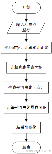
四、程序框图
五、完整代码
import matplotlib.pyplot as plt
import numpy as np
from scipy.interpolate import CubicSpline

def dms_to_decimal(degree, minutes): # 将度分(°′)格式转换为十进制度(°)格式
    return degree + minutes / 60

def convert_coordinates(coordinate_list):
    """
    将度分(°′)格式的坐标列表转换为十进制格式的坐标列表
    :param coordinate_list: 度分格式的坐标列表,例如 [(15, 8.1, 117, 50.9), ...]
    :return: 十进制格式的坐标列表
    """
    decimal_coords = []
    for lat_deg, lat_min, lon_deg, lon_min in coordinate_list:
        lat_decimal = dms_to_decimal(lat_deg, lat_min)
        lon_decimal = dms_to_decimal(lon_deg, lon_min)
        decimal_coords.append((lat_decimal, lon_decimal))
    return decimal_coords


def polygon_area(coords):
    """
    使用鞋带公式计算多边形的面积(单位:平方度)
    :param coords: 经纬度坐标元组列表
    :return: 多边形的面积(单位:平方公里)
    """
    # 将经纬度转换为平面坐标系(近似)
    latitudes, longitudes = zip(*coords)
    latitudes = np.radians(latitudes)
    longitudes = np.radians(longitudes)

    # 计算多边形面积
    area = 0
    n = len(coords)
    for i in range(n):
        j = (i + 1) % n
        area += longitudes[i] * latitudes[j]
        area -= longitudes[j] * latitudes[i]

    area = abs(area) / 2.0

    # 由于是球面面积,调整单位为平方公里
    R = 6371  # 地球半径(单位:公里)
    area = area * R ** 2  # 单位:平方公里

    return area

def smooth_coordinates(coords, num_points=500):
    """
    使用三次样条插值平滑坐标点
    :param coords: 原始坐标点列表
    :param num_points: 平滑后生成的点数量
    :return: 平滑后的坐标列表
    """
    latitudes, longitudes = zip(*coords)

    # 去掉最后一个重复点
    latitudes = np.array(latitudes[:-1])
    longitudes = np.array(longitudes[:-1])

    # 计算累积距离(作为插值的自变量)
    distances = np.sqrt(np.diff(latitudes)**2 + np.diff(longitudes)**2)
    cumulative_distances = np.insert(np.cumsum(distances), 0, 0)

    # 三次样条插值
    cs_lat = CubicSpline(cumulative_distances, latitudes)
    cs_lon = CubicSpline(cumulative_distances, longitudes)

    # 在均匀分布的插值点上计算平滑结果
    interp_distances = np.linspace(0, cumulative_distances[-1], num_points)
    smooth_latitudes = cs_lat(interp_distances)
    smooth_longitudes = cs_lon(interp_distances)

    # 添加首尾点使曲线闭合
    smooth_latitudes = np.append(smooth_latitudes, smooth_latitudes[0])
    smooth_longitudes = np.append(smooth_longitudes, smooth_longitudes[0])

    # 返回平滑后的坐标
    return list(zip(smooth_latitudes, smooth_longitudes))


# 标志点坐标:每个坐标是(纬度度数, 纬度分数, 经度度数, 经度分数)
coordinate_list = [
    (15, 8.1, 117, 50.9),
    (15, 7.4, 117, 50.8),
    (15, 7.0, 117, 50.6),
    (15, 6.6, 117, 50.2),
    (15, 6.1, 117, 49.5),
    (15, 6.3, 117, 44.2),
    (15, 7.3, 117, 43.1),
    (15, 12.7, 117, 42.6),
    (15, 13.1, 117, 42.8),
    (15, 13.4, 117, 43.3),
    (15, 13.5, 117, 43.9),
    (15, 13.5, 117, 44.4),
    (15, 9.6, 117, 49.7),
    (15, 9.0, 117, 50.4),
    (15, 8.5, 117, 50.8),
    (15, 8.1, 117, 50.9)
]
# 转换为十进制格式
coords = convert_coordinates(coordinate_list)

# 计算直线连接的面积
straight_area = polygon_area(coords)

# 平滑坐标并计算面积
smooth_coords = smooth_coordinates(coords)
smooth_area = polygon_area(smooth_coords)

# 计算面积差
area_difference = abs(smooth_area - straight_area)

# 提取直线坐标和平滑曲线坐标
straight_latitudes = [coord[0] for coord in coords]
straight_longitudes = [coord[1] for coord in coords]
smooth_latitudes = [coord[0] for coord in smooth_coords]
smooth_longitudes = [coord[1] for coord in smooth_coords]

# 创建一个图形
plt.figure(figsize=(10, 8))

# 设置字体,避免中文显示问题
plt.rcParams['font.sans-serif'] = ['SimHei']  # 设置中文字体
plt.rcParams['axes.unicode_minus'] = False  # 解决负号显示问题

# 绘制直线连接的边界
plt.plot(straight_longitudes, straight_latitudes, marker='o', color='b', linestyle='-', markersize=5, label='直线连接边界')

# 绘制平滑曲线连接的边界
plt.plot(smooth_longitudes, smooth_latitudes, color='r', linestyle='--', label='平滑曲线边界')

# 为每个点标注坐标
for i, (lat, lon) in enumerate(coords):
    plt.text(lon, lat, f'({lat:.2f}, {lon:.2f})', fontsize=8, ha='right')

# 设置标题和标签
plt.title("岛屿领海基线图")
plt.xlabel("经度")
plt.ylabel("纬度")

# 在图例下方显示面积信息
props = dict(boxstyle='round', facecolor='white', alpha=0.8)
plt.text(0.72, 0.82, f"直线连接面积: {straight_area:.2f} 平方公里\n"
                     f"平滑曲线面积: {smooth_area:.2f} 平方公里\n"
                     f"面积差: {area_difference:.2f} 平方公里",
         transform=plt.gca().transAxes, fontsize=10, color="black", ha='left', bbox=props)

plt.grid(True) # 显示网格
plt.legend(loc="upper right")  # 显示图例

plt.show() # 显示图形
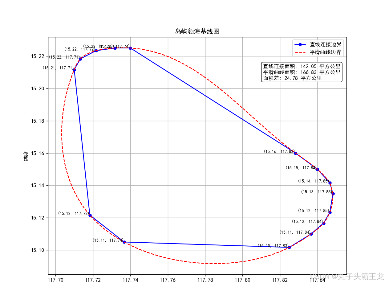
六、结果展示
运行代码计算出直线连接的岛屿领海基线围起来的面积是142.05平方公里,而平滑曲线连接的面积是166.83平方公里,二者相差24.78平方公里。直线连接和平滑曲线连接的示意图如图所示。


 3191
3191

 被折叠的 条评论
为什么被折叠?
被折叠的 条评论
为什么被折叠?
 到【灌水乐园】发言


