minepy 包——基于最大信息的非参数估计

简介

minepy 提供 ANSI C 库的基于最大信息的非参数估计的实现（Maximal Information-based Nonparametric Exploration,MIC and MINE family).

特点

APPROX-MIC (the original algorithm, DOI: 10.1126/science.1205438) and MIC_e (DOI: arXiv:1505.02213 and DOI: arXiv:1505.02214) estimators;
Total Information Coefficient (TIC, DOI: arXiv:1505.02213) and the Generalized Mean Information Coefficient (GMIC, DOI: arXiv:1308.5712);
C++接口 ;
Python 接口;
MATLAB/OCTAVE API;
和原生的MINE.jar相似的命令行工具;
R 接口 CRAN.

Python API

class minepy.MINE(alpha=0.6, c=15, est="mic_approx")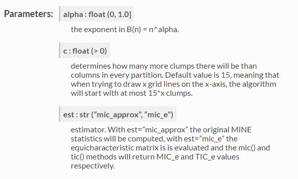

这里写图片描述

示例代码

import numpy as np
from minepy import MINE

def print_stats(mine):
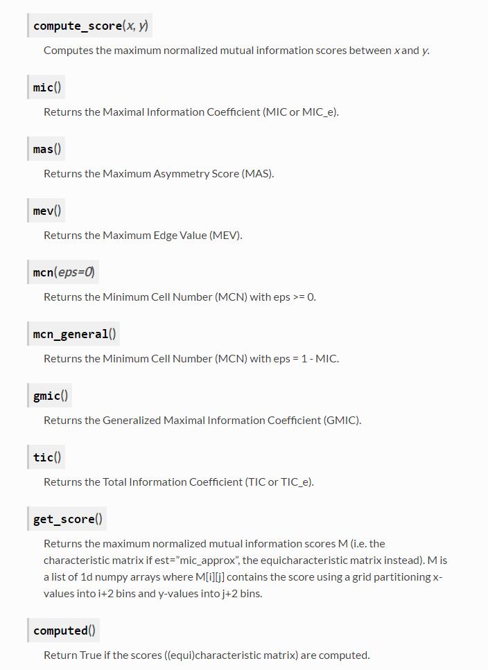
    print "MIC", mine.mic()
    print "MAS", mine.mas()
    print "MEV", mine.mev()
    print "MCN (eps=0)", mine.mcn(0)
    print "MCN (eps=1-MIC)", mine.mcn_general()
    print "GMIC", mine.gmic()
    print "TIC", mine.tic()

x = np.linspace(0, 1, 1000)
y = np.sin(10 * np.pi * x) + x
mine = MINE(alpha=0.6, c=15, est="mic_approx")
mine.compute_score(x, y)

print "Without noise:"
print_stats(mine)
print

np.random.seed(0)
y +=np.random.uniform(-1, 1, x.shape[0]) # add some noise
mine.compute_score(x, y)

print "With noise:"
print_stats(mine)

运行结果

$ python python_example.py
Without noise:
MIC 1.0
MAS 0.726071574374
MEV 1.0
MCN (eps=0) 4.58496250072
MCN (eps=1-MIC) 4.58496250072
GMIC 0.779360251901
TIC 67.6612295532

With noise:
MIC 0.505716693417
MAS 0.365399904262
MEV 0.505716693417
MCN (eps=0) 5.95419631039
MCN (eps=1-MIC) 3.80735492206
GMIC 0.359475501353
TIC 28.7498326953

from __future__ import division
import numpy as np
import matplotlib.pyplot as plt
from minepy import MINE


rs = np.random.RandomState(seed=0)

def mysubplot(x, y, numRows, numCols, plotNum,
              xlim=(-4, 4), ylim=(-4, 4)):

    r = np.around(np.corrcoef(x, y)[0, 1], 1)
    mine = MINE(alpha=0.6, c=15, est="mic_approx")
    mine.compute_score(x, y)
    mic = np.around(mine.mic(), 1)
    ax = plt.subplot(numRows, numCols, plotNum,
                     xlim=xlim, ylim=ylim)
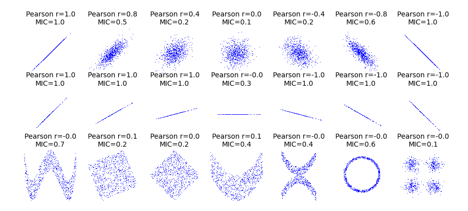
    ax.set_title('Pearson r=%.1f\nMIC=%.1f' % (r, mic),fontsize=10)
    ax.set_frame_on(False)
    ax.axes.get_xaxis().set_visible(False)
    ax.axes.get_yaxis().set_visible(False)
    ax.plot(x, y, ',')
    ax.set_xticks([])
    ax.set_yticks([])
    return ax

def rotation(xy, t):
    return np.dot(xy, [[np.cos(t), -np.sin(t)], [np.sin(t), np.cos(t)]])

def mvnormal(n=1000):
    cors = [1.0, 0.8, 0.4, 0.0, -0.4, -0.8, -1.0]
    for i, cor in enumerate(cors):
        cov = [[1, cor],[cor, 1]]
        xy = rs.multivariate_normal([0, 0], cov, n)
        mysubplot(xy[:, 0], xy[:, 1], 3, 7, i+1)

def rotnormal(n=1000):
    ts = [0, np.pi/12, np.pi/6, np.pi/4, np.pi/2-np.pi/6,
          np.pi/2-np.pi/12, np.pi/2]
    cov = [[1, 1],[1, 1]]
    xy = rs.multivariate_normal([0, 0], cov, n)
    for i, t in enumerate(ts):
        xy_r = rotation(xy, t)
        mysubplot(xy_r[:, 0], xy_r[:, 1], 3, 7, i+8)

def others(n=1000):
    x = rs.uniform(-1, 1, n)
    y = 4*(x**2-0.5)**2 + rs.uniform(-1, 1, n)/3
    mysubplot(x, y, 3, 7, 15, (-1, 1), (-1/3, 1+1/3))

    y = rs.uniform(-1, 1, n)
    xy = np.concatenate((x.reshape(-1, 1), y.reshape(-1, 1)), axis=1)
    xy = rotation(xy, -np.pi/8)
    lim = np.sqrt(2+np.sqrt(2)) / np.sqrt(2)
    mysubplot(xy[:, 0], xy[:, 1], 3, 7, 16, (-lim, lim), (-lim, lim))

    xy = rotation(xy, -np.pi/8)
    lim = np.sqrt(2)
    mysubplot(xy[:, 0], xy[:, 1], 3, 7, 17, (-lim, lim), (-lim, lim))

    y = 2*x**2 + rs.uniform(-1, 1, n)
    mysubplot(x, y, 3, 7, 18, (-1, 1), (-1, 3))

    y = (x**2 + rs.uniform(0, 0.5, n)) * \
        np.array([-1, 1])[rs.random_integers(0, 1, size=n)]
    mysubplot(x, y, 3, 7, 19, (-1.5, 1.5), (-1.5, 1.5))

    y = np.cos(x * np.pi) + rs.uniform(0, 1/8, n)
    x = np.sin(x * np.pi) + rs.uniform(0, 1/8, n)
    mysubplot(x, y, 3, 7, 20, (-1.5, 1.5), (-1.5, 1.5))

    xy1 = np.random.multivariate_normal([3, 3], [[1, 0], [0, 1]], int(n/4))
    xy2 = np.random.multivariate_normal([-3, 3], [[1, 0], [0, 1]], int(n/4))
    xy3 = np.random.multivariate_normal([-3, -3], [[1, 0], [0, 1]], int(n/4))
    xy4 = np.random.multivariate_normal([3, -3], [[1, 0], [0, 1]], int(n/4))
    xy = np.concatenate((xy1, xy2, xy3, xy4), axis=0)
    mysubplot(xy[:, 0], xy[:, 1], 3, 7, 21, (-7, 7), (-7, 7))

plt.figure(facecolor='white')
mvnormal(n=800)
rotnormal(n=200)
others(n=800)
plt.tight_layout()
plt.show()